library(bayesrules)
library(tidyverse)
library(brms)
library(cmdstanr)
library(rstanarm)
library(broom.mixed)
library(tidybayes)
library(ggdist)
library(patchwork)

# Plot stuff
clrs <- MetBrewer::met.brewer("Lakota", 6)
theme_set(theme_bw())

# Seed stuff
set.seed(1234)
BAYES_SEED <- 1234

data(weather_WU, package = "bayesrules")

weather_WU <- weather_WU %>%
  select(location, windspeed9am, humidity9am, pressure9am, temp9am, temp3pm) |>
  mutate(across(c(temp9am, temp3pm, humidity9am, windspeed9am, pressure9am),
                ~scale(., scale = FALSE), .names = "{col}_centered")) |>
  mutate(across(c(temp9am, temp3pm, humidity9am, windspeed9am, pressure9am),
                ~as.numeric(scale(., scale = FALSE)), .names = "{col}_c"))

extract_attributes <- function(x) {
  attributes(x) %>%
    set_names(janitor::make_clean_names(names(.))) %>%
    as_tibble() %>%
    slice(1)
}

unscaled <- weather_WU %>%
  select(ends_with("_centered")) |>
  summarize(across(everything(), ~extract_attributes(.))) |>
  pivot_longer(everything()) |>
  unnest(value) |>
  split(~name)

# Access these things like so:
# unscaled$temp3pm_centered$scaled_center11: Extending the normal regression model
Reading notes
The general setup
We want to know the relationship between morning and afternoon temperatures in Wollongong and Uluru:
ggplot(weather_WU, aes(x = temp9am, y = temp3pm)) +
  geom_point()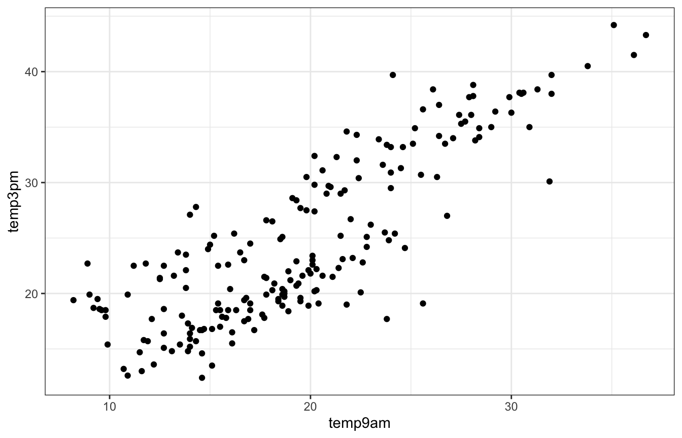
Looks linear enough. Let’s make a model with vague priors (just in rstanarm and brms for now; no need for raw Stan here):
\[ \begin{aligned} Y_i \mid \beta_0, \beta_1, \beta_2, \sigma &\stackrel{\text{ind}}{\sim} \mathcal{N}(\mu_i, \sigma^2) \\ \mu_i &= \beta_{0c} + \beta_1 X_{i1} \\ \\ \beta_{0c} &\sim \mathcal{N}(25, 5) \\ \beta_{1} &\sim \mathcal{N}(0, 2.5) \\ \sigma &\sim \operatorname{Exponential}(1) \end{aligned} \]
weather_simple_rstanarm <- stan_glm(
  temp3pm ~ temp9am,
  data = weather_WU,
  family = gaussian(),
  prior_intercept = normal(25, 5),
  prior = normal(0, 2.5, autoscale = TRUE),
  prior_aux = exponential(1, autoscale = TRUE),
  chains = 4, iter = 5000*2, seed = 84735, refresh = 0
)
priors <- c(prior(normal(25, 5), class = Intercept),
prior(normal(0, 2.5), class = b, coef = "temp9am"),
prior(exponential(1), class = sigma))
weather_simple_brms <- brm(
bf(temp3pm ~ temp9am),
data = weather_WU,
family = gaussian(),
prior = priors,
chains = 4, iter = 5000*2, seed = BAYES_SEED,
backend = "cmdstanr", refresh = 0
)
## Start samplingWe’ll skip all the diagnostics for now—they cover them in the book. What really matters is how well this model fits the data, and it’s not great. We’ve got a weird hump in the data that’s not accounted for in the model. We’ve got to do something about that.
pp_check(weather_simple_brms, ndraws = 25)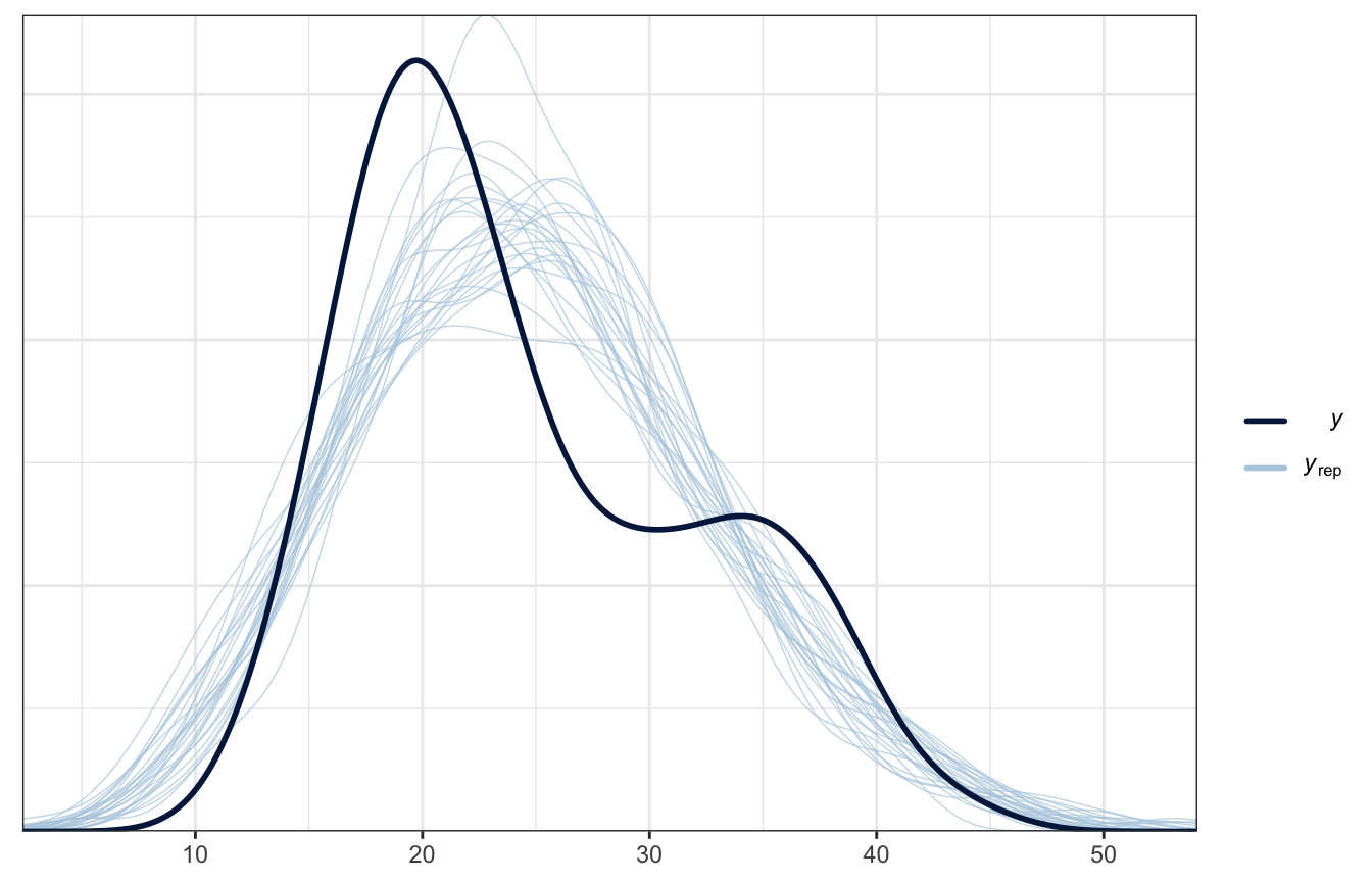
Note
I went into super detail in chapters 9 and 10, with examples in rstanarm, brms, and raw Stan, and with manual calculation of core Bayesian things, like posterior predictive checks, k-fold cross validation, and a bunch of other things.
I don’t do that in this chapter, since I’ve been doing Bayesian regression stuff for years. Here I just do rstanarm and brms versions of everything and pre-written checks like pp_check(); no raw Stan here.
11.1: Utilizing a categorical predictor
What if we just use location to predict afternoon temperatures? It’s an important factor:
ggplot(weather_WU, aes(x = temp3pm, fill = location)) +
  geom_density(color = NA) +
  scale_fill_manual(values = c(clrs[2], clrs[1])) +
  labs(x = "3 PM temperature", fill = NULL)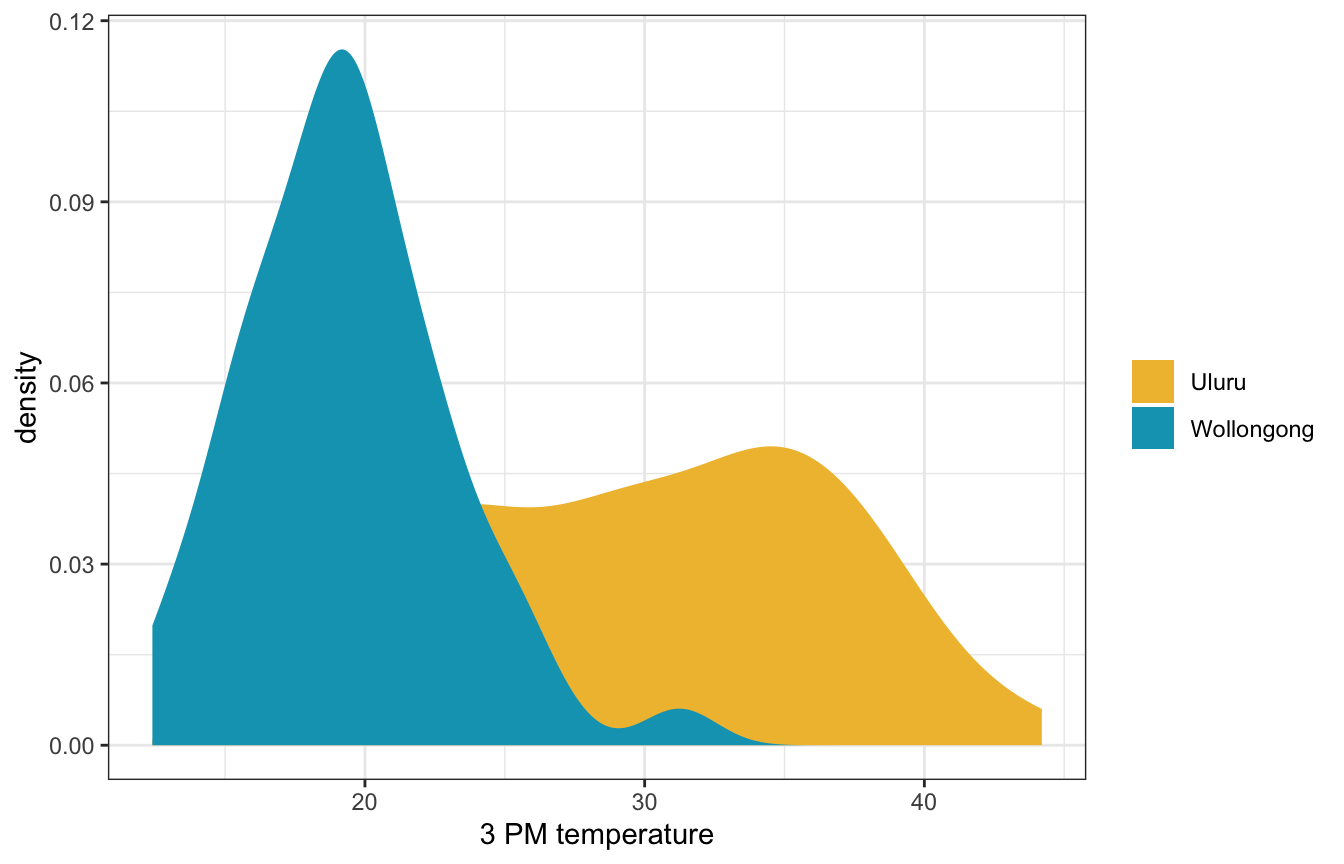
We can include it as a term in the model:
\[ \begin{aligned} Y_i \mid \beta_0, \beta_1, \sigma &\stackrel{\text{ind}}{\sim} \mathcal{N}(\mu_i, \sigma^2) \\ \mu_i &= \beta_{0c} + \beta_1 X_{i1} \\ \\ \beta_{0c} &\sim \mathcal{N}(25, 5) \\ \beta_{1} &\sim \mathcal{N}(0, 10) \\ \sigma &\sim \operatorname{Exponential}(1) \end{aligned} \]
Understanding the priors
These all look reasonable.
weather_location_only_prior_rstanarm <- stan_glm(
  temp3pm ~ location,
  data = weather_WU,
  family = gaussian,
  prior_intercept = normal(25, 5),
  prior = normal(0, 2.5, autoscale = TRUE),
  prior_aux = exponential(1, autoscale = TRUE),
  chains = 4, iter = 5000*2, seed = 84735, refresh = 0,
  prior_PD = TRUE
)
weather_WU |>
add_predicted_draws(weather_location_only_prior_rstanarm, ndraws = 100) |>
ggplot(aes(x = .prediction, group = .draw)) +
geom_density(size = 0.25, color = clrs[3]) +
labs(x = "Predicted 3 PM temperature", y = "Density")
## Warning: Using `size` aesthetic for lines was deprecated in ggplot2 3.4.0.
## ℹ Please use `linewidth` instead.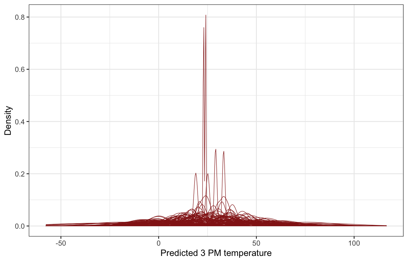
priors <- c(prior(normal(25, 5), class = Intercept),
            prior(normal(0, 10), class = b, coef = "locationWollongong"),
            prior(exponential(1), class = sigma))

weather_location_only_prior_brms <- brm(
  bf(temp3pm ~ location),
  data = weather_WU,
  family = gaussian(),
  prior = priors,
  chains = 4, iter = 5000*2, seed = BAYES_SEED,
  backend = "cmdstanr", refresh = 0,
  sample_prior = "only"
)
## Start sampling
weather_WU |>
add_predicted_draws(weather_location_only_prior_brms, ndraws = 100) |>
ggplot(aes(x = .prediction, group = .draw)) +
geom_density(size = 0.25, color = clrs[3]) +
labs(x = "Predicted 3 PM temperature", y = "Density")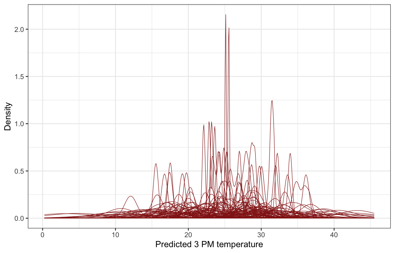
Simulating the posterior
Model
weather_location_only_rstanarm <- stan_glm(
  temp3pm ~ location,
  data = weather_WU,
  family = gaussian,
  prior_intercept = normal(25, 5),
  prior = normal(0, 2.5, autoscale = TRUE),
  prior_aux = exponential(1, autoscale = TRUE),
  chains = 4, iter = 5000*2, seed = 84735, refresh = 0
)tidy(weather_location_only_rstanarm, effects = c("fixed", "aux"),
conf.int = TRUE, conf.level = 0.8)
## # A tibble: 4 × 5
## term estimate std.error conf.low conf.high
## <chr> <dbl> <dbl> <dbl> <dbl>
## 1 (Intercept) 29.7 0.548 29.0 30.4
## 2 locationWollongong -10.3 0.777 -11.3 -9.30
## 3 sigma 5.48 0.279 5.14 5.86
## 4 mean_PPD 24.6 0.547 23.9 25.3Coefficient posteriors
weather_location_only_rstanarm |>
  gather_draws(`(Intercept)`, locationWollongong, sigma) |>
  ggplot(aes(x = .value, fill = .variable)) +
  stat_halfeye(normalize = "xy") +
  scale_fill_manual(values = c(clrs[1], clrs[3], clrs[4]), guide = "none") +
  facet_wrap(vars(.variable), scales = "free_x") +
  labs(x = "Parameter posterior") +
  theme(legend.position = "bottom")
## Warning: Unknown or uninitialised column: `linewidth`.
## Warning: Using the `size` aesthietic with geom_segment was deprecated in ggplot2 3.4.0.
## ℹ Please use the `linewidth` aesthetic instead.
## Warning: Unknown or uninitialised column: `linewidth`.
## Unknown or uninitialised column: `linewidth`.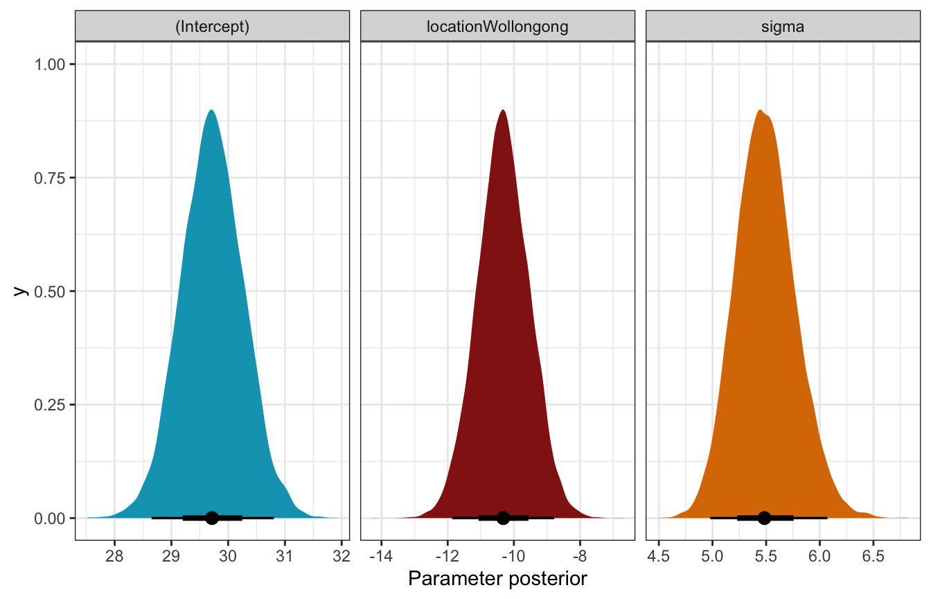
Posterior predictive check
Ew!
pp_check(weather_location_only_rstanarm, n = 25)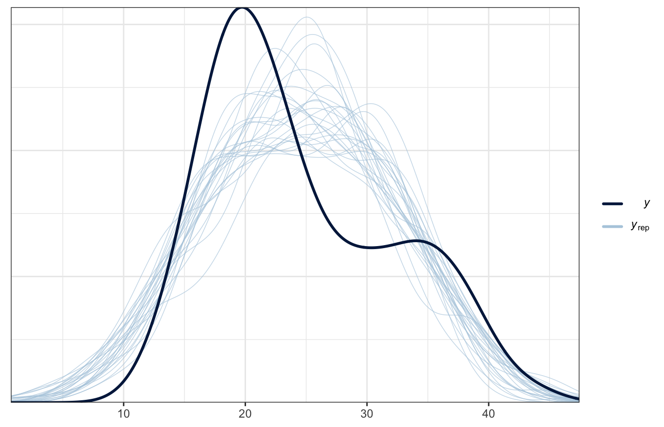
Model
priors <- c(prior(normal(25, 5), class = Intercept),
            prior(normal(0, 10), class = b, coef = "locationWollongong"),
            prior(exponential(1), class = sigma))

weather_location_only_brms <- brm(
  bf(temp3pm ~ location),
  data = weather_WU,
  family = gaussian(),
  prior = priors,
  chains = 4, iter = 5000*2, seed = BAYES_SEED,
  backend = "cmdstanr", refresh = 0
)
## Start samplingtidy(weather_location_only_brms, conf.int = TRUE, conf.level = 0.8) |>
select(-c(effect, component, group))
## # A tibble: 3 × 5
## term estimate std.error conf.low conf.high
## <chr> <dbl> <dbl> <dbl> <dbl>
## 1 (Intercept) 29.7 0.544 29.0 30.4
## 2 locationWollongong -10.3 0.762 -11.2 -9.29
## 3 sd__Observation 5.44 0.272 5.10 5.79Coefficient posteriors
weather_location_only_brms |>
  gather_draws(b_Intercept, b_locationWollongong, sigma) |>
  ggplot(aes(x = .value, fill = .variable)) +
  stat_halfeye(normalize = "xy") +
  scale_fill_manual(values = c(clrs[1], clrs[3], clrs[4]), guide = "none") +
  facet_wrap(vars(.variable), scales = "free_x") +
  labs(x = "Parameter posterior") +
  theme(legend.position = "bottom")
## Warning: Unknown or uninitialised column: `linewidth`.
## Unknown or uninitialised column: `linewidth`.
## Unknown or uninitialised column: `linewidth`.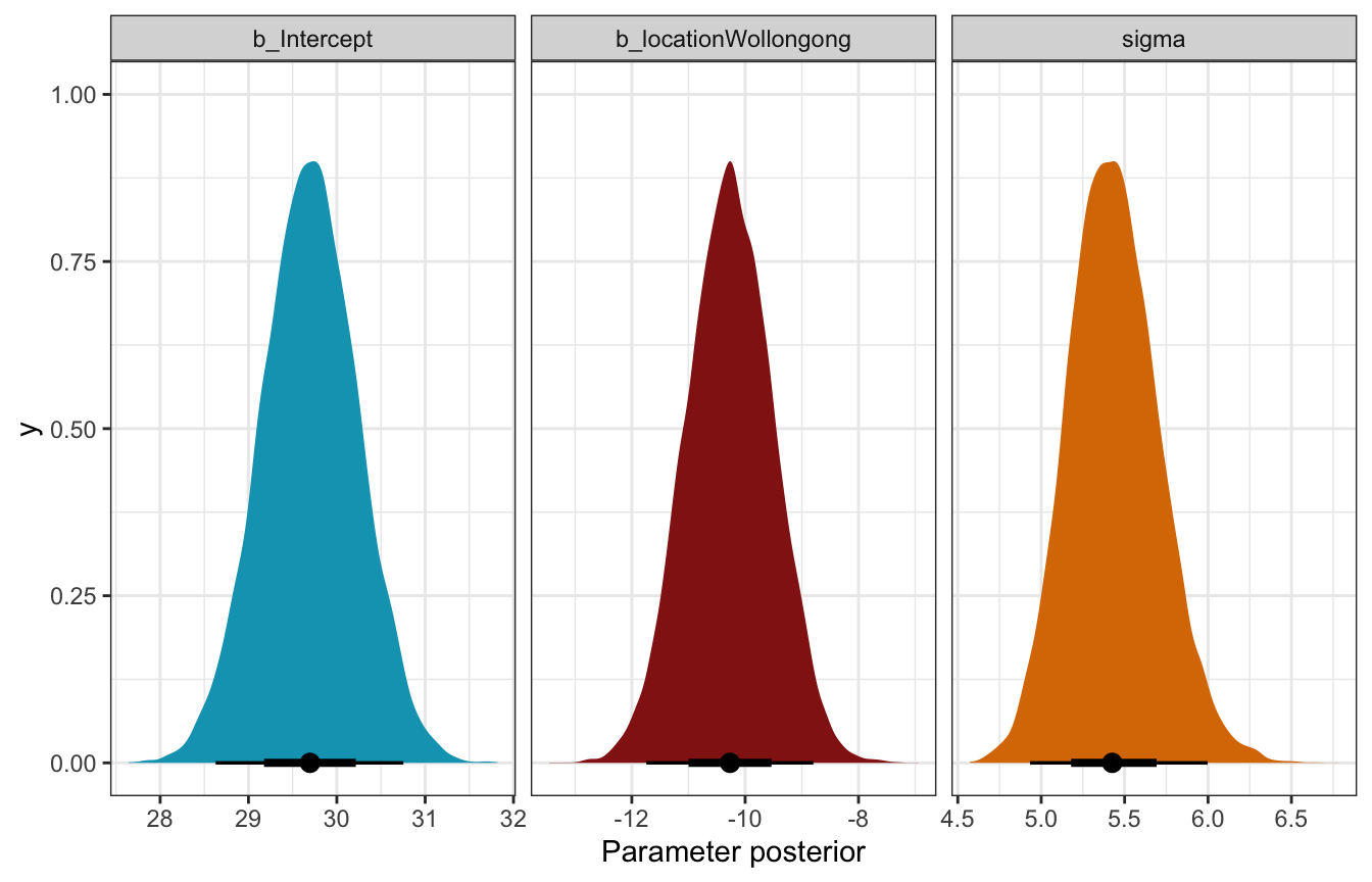
Posterior predictive check
Not great!
pp_check(weather_location_only_brms, ndraws = 25)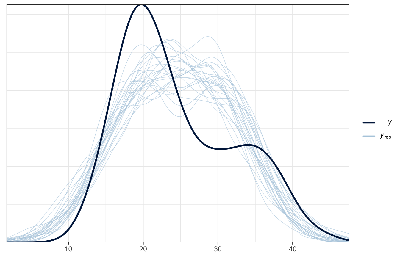
Posterior prediction
What’s the predicted afternoon temperature in these two cities?
weather_location_only_rstanarm |>
  predicted_draws(newdata = tibble(location = c("Wollongong", "Uluru"))) |>
  ggplot(aes(x = .prediction, y = location, fill = location)) +
  stat_halfeye() +
  scale_fill_manual(values = c(clrs[2], clrs[1]), guide = "none") +
  labs(x = "Predicted 3 PM temperature", y = NULL)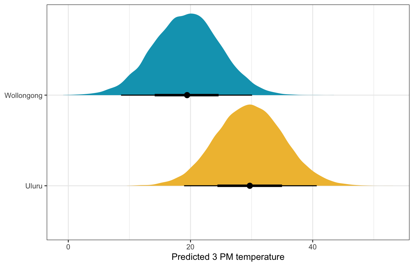
weather_location_only_brms |>
  predicted_draws(newdata = tibble(location = c("Wollongong", "Uluru"))) |>
  ggplot(aes(x = .prediction, y = location, fill = location)) +
  stat_halfeye() +
  scale_fill_manual(values = c(clrs[2], clrs[1]), guide = "none") +
  labs(x = "Predicted 3 PM temperature", y = NULL)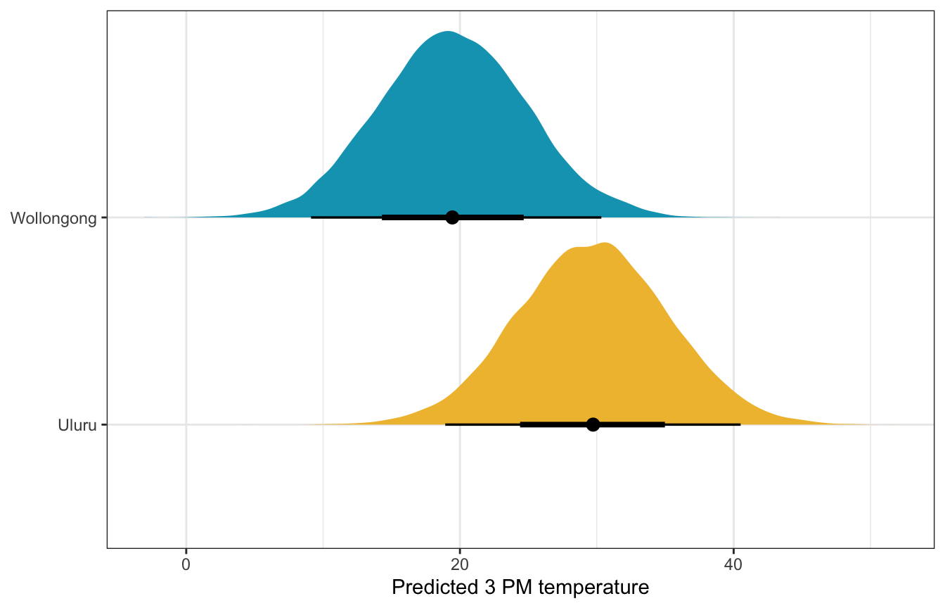
11.2: Utilizing two predictors
There’s a recognizable cluster in the data here: location. Wollongong has lower afternoon temperatures than Uluru. That makes sense—Wollongong is a coastal city near Sydney and Uluru is right in the middle of Australia in the desert.
ggplot(weather_WU, aes(x = temp9am, y = temp3pm, color = location)) +
  geom_point() +
  geom_smooth(method = "lm", se = FALSE) +
  scale_color_manual(values = c(clrs[2], clrs[1])) +
  labs(x = "9 AM temperature", y = "3 PM temperature", color = NULL)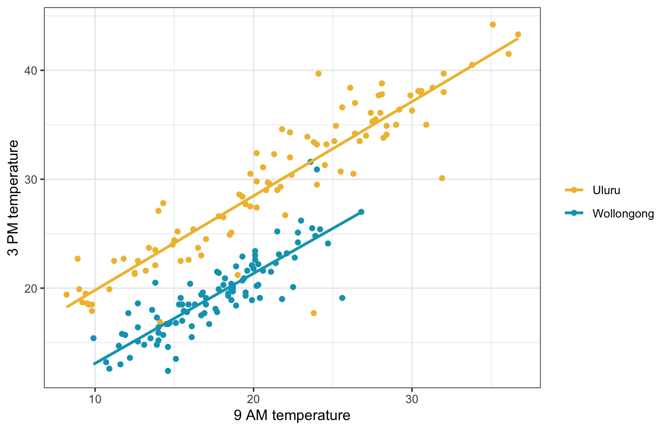
Since location is binary, including it as a covariate will shift the intercept up and down
\[ \begin{aligned} Y_i \mid \beta_0, \beta_1, \beta_2, \sigma &\stackrel{\text{ind}}{\sim} \mathcal{N}(\mu_i, \sigma^2) \\ \mu_i &= \beta_{0c} + \beta_1 X_{i1} + \beta_2 X_{i2} \\ \\ \beta_{0c} &\sim \mathcal{N}(25, 5) \\ \beta_{1} &\sim \mathcal{N}(0, 2.5) \\ \beta_{2} &\sim \mathcal{N}(0, 10) \\ \sigma &\sim \operatorname{Exponential}(1) \end{aligned} \]
Understanding the priors
These all look reasonable.
weather_location_prior_rstanarm <- stan_glm(
  temp3pm ~ temp9am + location,
  data = weather_WU,
  family = gaussian,
  prior_intercept = normal(25, 5),
  prior = normal(0, 2.5, autoscale = TRUE),
  prior_aux = exponential(1, autoscale = TRUE),
  chains = 4, iter = 5000*2, seed = 84735, refresh = 0,
  prior_PD = TRUE
)
p1 <- weather_WU |>
add_predicted_draws(weather_location_prior_rstanarm, ndraws = 100) |>
ggplot(aes(x = .prediction, group = .draw)) +
geom_density(size = 0.25, color = clrs[3]) +
labs(x = "Predicted 3 PM temperature", y = "Density")
# Feed add_epred_draws() brand new data instead of the original data, just for fun
prior_draws_rstanarm <- weather_WU |>
group_by(location) |>
summarize(min = min(temp9am),
max = max(temp9am)) |>
mutate(temp9am = map2(min, max, ~seq(.x, .y, 1))) |>
unnest(temp9am) |>
add_epred_draws(weather_location_prior_rstanarm, ndraws = 100)
p2 <- prior_draws_rstanarm |>
ggplot(aes(x = temp9am, y = .epred)) +
geom_line(aes(group = paste(location, .draw), color = location), alpha = 0.2) +
scale_color_manual(values = c(clrs[2], clrs[1])) +
labs(x = "9 AM temperature", y = "3 PM temperature", color = NULL) +
theme(legend.position = "bottom")
p1 | p2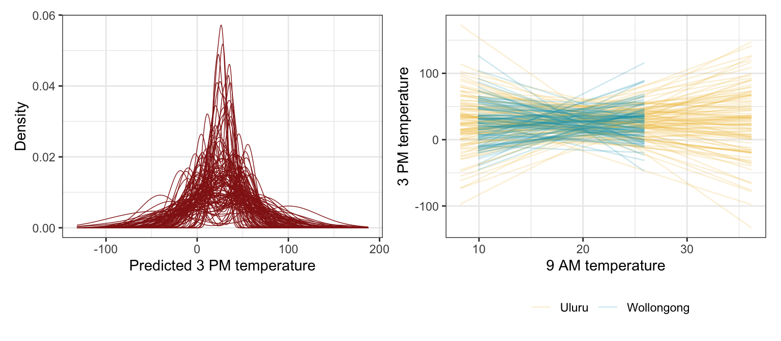
priors <- c(prior(normal(25, 5), class = Intercept),
            prior(normal(0, 2.5), class = b, coef = "temp9am_c"),
            prior(normal(0, 10), class = b, coef = "locationWollongong"),
            prior(exponential(1), class = sigma))

weather_location_prior_brms <- brm(
  bf(temp3pm ~ temp9am_c + location),
  data = weather_WU,
  family = gaussian(),
  prior = priors,
  chains = 4, iter = 5000*2, seed = BAYES_SEED,
  backend = "cmdstanr", refresh = 0,
  sample_prior = "only"
)
## Start sampling
p1 <- weather_WU |>
add_predicted_draws(weather_location_prior_brms, ndraws = 100) |>
ggplot(aes(x = .prediction, group = .draw)) +
geom_density(size = 0.25, color = clrs[3]) +
labs(x = "Predicted 3 PM temperature", y = "Density")
# Feed add_epred_draws() brand new data instead of the original data, just for fun
prior_draws_brms <- weather_WU |>
group_by(location) |>
summarize(min = min(temp9am_c),
max = max(temp9am_c)) |>
mutate(temp9am_c = map2(min, max, ~seq(.x, .y, 1))) |>
unnest(temp9am_c) |>
add_epred_draws(weather_location_prior_brms, ndraws = 100) |>
mutate(temp9am = temp9am_c + unscaled$temp9am_centered$scaled_center)
p2 <- prior_draws_brms |>
ggplot(aes(x = temp9am, y = .epred)) +
geom_line(aes(group = paste(location, .draw), color = location), alpha = 0.2) +
scale_color_manual(values = c(clrs[2], clrs[1])) +
labs(x = "9 AM temperature", y = "3 PM temperature", color = NULL) +
theme(legend.position = "bottom")
p1 | p2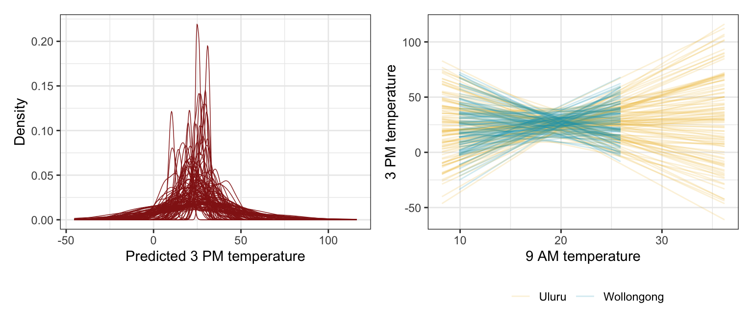
Simulating the posterior
Model
weather_location_rstanarm <- stan_glm(
  temp3pm ~ temp9am + location,
  data = weather_WU,
  family = gaussian,
  prior_intercept = normal(25, 5),
  prior = normal(0, 2.5, autoscale = TRUE),
  prior_aux = exponential(1, autoscale = TRUE),
  chains = 4, iter = 5000*2, seed = 84735, refresh = 0
)tidy(weather_location_rstanarm, effects = c("fixed", "aux"),
conf.int = TRUE, conf.level = 0.8)
## # A tibble: 5 × 5
## term estimate std.error conf.low conf.high
## <chr> <dbl> <dbl> <dbl> <dbl>
## 1 (Intercept) 11.3 0.671 10.5 12.2
## 2 temp9am 0.857 0.0291 0.820 0.895
## 3 locationWollongong -7.06 0.355 -7.51 -6.60
## 4 sigma 2.38 0.121 2.23 2.54
## 5 mean_PPD 24.6 0.236 24.3 24.9Coefficient posteriors
weather_location_rstanarm |>
  gather_draws(`(Intercept)`, temp9am, locationWollongong, sigma) |>
  ggplot(aes(x = .value, fill = .variable)) +
  stat_halfeye(normalize = "xy") +
  scale_fill_manual(values = c(clrs[1], clrs[3], clrs[4], clrs[5]), guide = "none") +
  facet_wrap(vars(.variable), scales = "free_x") +
  labs(x = "Parameter posterior") +
  theme(legend.position = "bottom")
## Warning: Unknown or uninitialised column: `linewidth`.
## Unknown or uninitialised column: `linewidth`.
## Unknown or uninitialised column: `linewidth`.
## Unknown or uninitialised column: `linewidth`.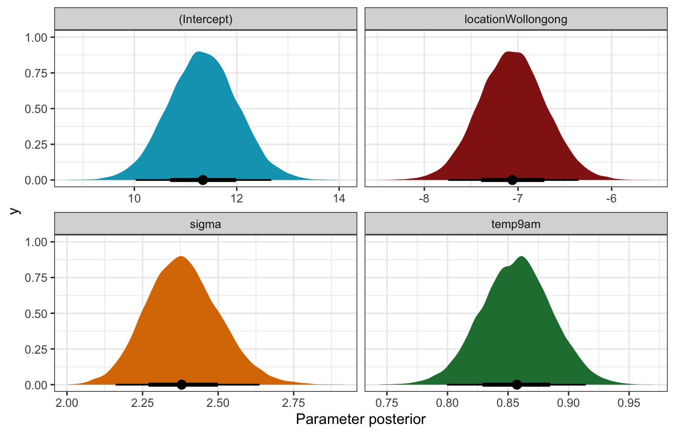
Fitted draws
weather_WU |>
  add_linpred_draws(weather_location_rstanarm, ndraws = 100) |>
  ggplot(aes(x = temp9am, y = temp3pm, color = location)) +
  geom_point(data = weather_WU, size = 0.5) +
  geom_line(aes(y = .linpred, group = paste(location, .draw)), alpha = 0.2, size = 0.5) +
  scale_color_manual(values = c(clrs[2], clrs[1])) +
  labs(x = "9 AM temperature", y = "3 PM temperature", color = NULL)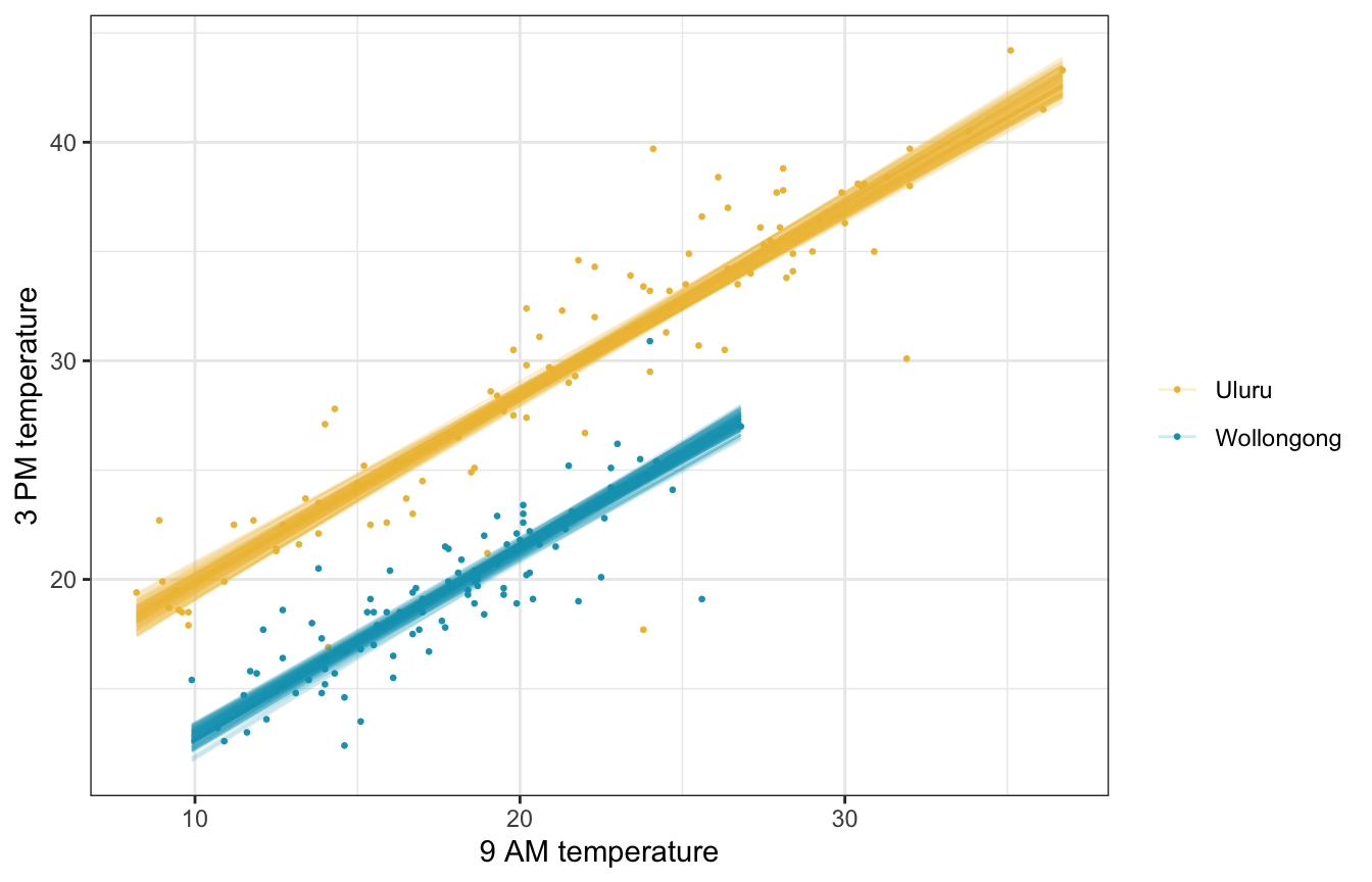
Posterior predictive check
Much better!
pp_check(weather_location_rstanarm, n = 25)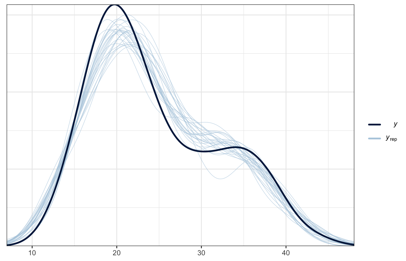
Model
priors <- c(prior(normal(25, 5), class = Intercept),
            prior(normal(0, 2.5), class = b, coef = "temp9am_c"),
            prior(normal(0, 10), class = b, coef = "locationWollongong"),
            prior(exponential(1), class = sigma))

weather_location_brms <- brm(
  bf(temp3pm ~ temp9am_c + location),
  data = weather_WU,
  family = gaussian(),
  prior = priors,
  chains = 4, iter = 5000*2, seed = BAYES_SEED,
  backend = "cmdstanr", refresh = 0
)
## Start samplingtidy(weather_location_brms, conf.int = TRUE, conf.level = 0.8) |>
select(-c(effect, component, group))
## Warning in tidy.brmsfit(weather_location_brms, conf.int = TRUE, conf.level =
## 0.8): some parameter names contain underscores: term naming may be unreliable!
## # A tibble: 4 × 5
## term estimate std.error conf.low conf.high
## <chr> <dbl> <dbl> <dbl> <dbl>
## 1 (Intercept) 28.1 0.243 27.8 28.4
## 2 temp9am_c 0.857 0.0294 0.820 0.895
## 3 locationWollongong -7.05 0.355 -7.50 -6.59
## 4 sd__Observation 2.37 0.119 2.23 2.53Coefficient posteriors
weather_location_brms |>
  gather_draws(b_Intercept, b_temp9am_c, b_locationWollongong, sigma) |>
  ggplot(aes(x = .value, fill = .variable)) +
  stat_halfeye(normalize = "xy") +
  scale_fill_manual(values = c(clrs[1], clrs[3], clrs[4], clrs[5]), guide = "none") +
  facet_wrap(vars(.variable), scales = "free_x") +
  labs(x = "Parameter posterior") +
  theme(legend.position = "bottom")
## Warning: Unknown or uninitialised column: `linewidth`.
## Unknown or uninitialised column: `linewidth`.
## Unknown or uninitialised column: `linewidth`.
## Unknown or uninitialised column: `linewidth`.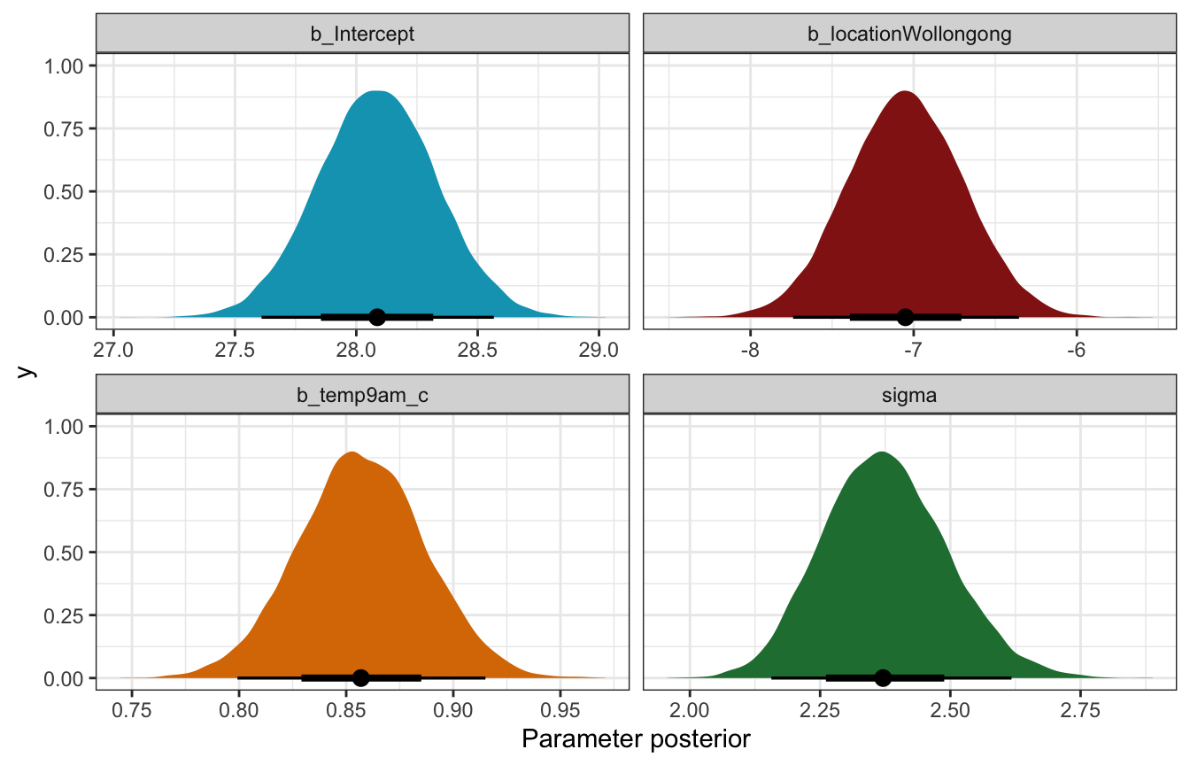
Fitted draws
weather_WU |>
  add_linpred_draws(weather_location_brms, ndraws = 100) |>
  ggplot(aes(x = temp9am, y = temp3pm, color = location)) +
  geom_point(data = weather_WU, size = 0.5) +
  geom_line(aes(y = .linpred, group = paste(location, .draw)), alpha = 0.2, size = 0.5) +
  scale_color_manual(values = c(clrs[2], clrs[1])) +
  labs(x = "9 AM temperature", y = "3 PM temperature", color = NULL)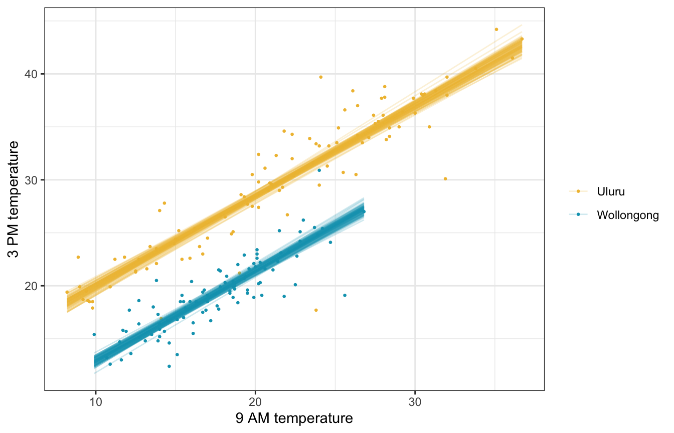
Posterior predictive check
Much better!
pp_check(weather_location_brms, ndraws = 25)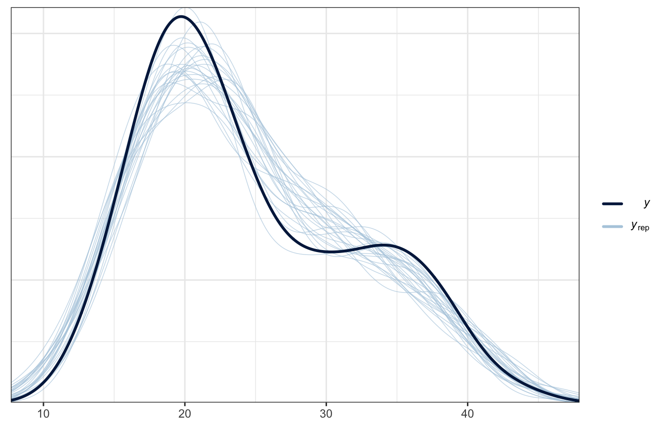
Posterior prediction
What if it’s 10˚ at 9 AM in both cities? What’s the predicted afternoon temperature?
weather_location_rstanarm |>
  predicted_draws(newdata = expand_grid(temp9am = 10,
                                        location = c("Wollongong", "Uluru"))) |>
  ggplot(aes(x = .prediction, y = location, fill = location)) +
  stat_halfeye() +
  scale_fill_manual(values = c(clrs[2], clrs[1]), guide = "none") +
  labs(x = "Predicted 3 PM temperature", y = NULL)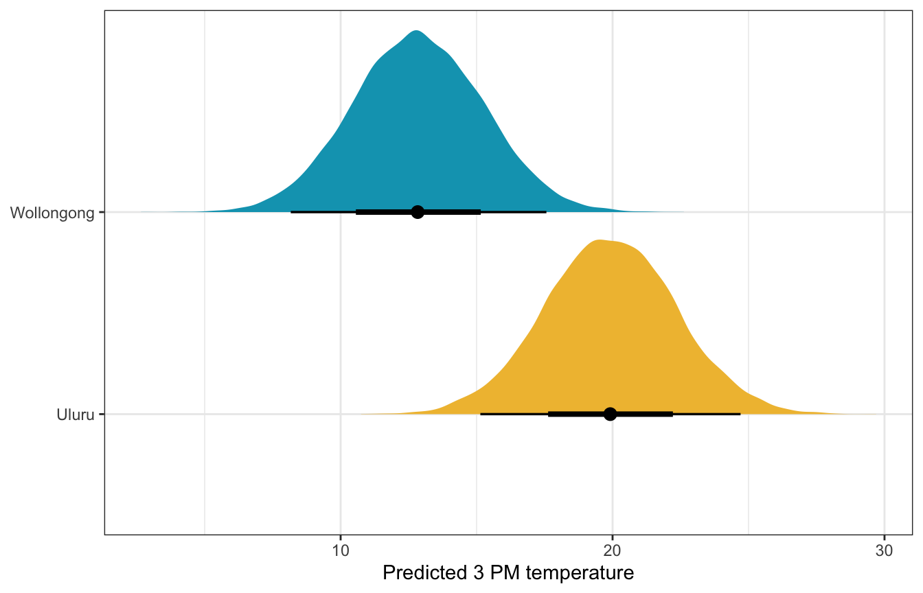
weather_location_brms |>
  predicted_draws(newdata = expand_grid(temp9am_c = 10 - unscaled$temp9am_centered$scaled_center,
                                        location = c("Wollongong", "Uluru"))) |>
  ggplot(aes(x = .prediction, y = location, fill = location)) +
  stat_halfeye() +
  scale_fill_manual(values = c(clrs[2], clrs[1]), guide = "none") +
  labs(x = "Predicted 3 PM temperature", y = NULL)
11.3: Utilizing interaction terms
Using location as an indicator variable made sense for 9 AM temperatures—the relationship was the same in both locations, but one was just shifted up compared to the other. But that’s not always the case! Here’s 9 AM humidity. It’s wildly different across the two locations (again because Uluru is in the middle of the desert and Wollongong is on the coast).
ggplot(weather_WU, aes(x = humidity9am, y = temp3pm, color = location)) +
  geom_point() +
  geom_smooth(method = "lm", se = FALSE) +
  scale_color_manual(values = c(clrs[2], clrs[1])) +
  labs(x = "9 AM humidity", y = "3 PM temperature", color = NULL)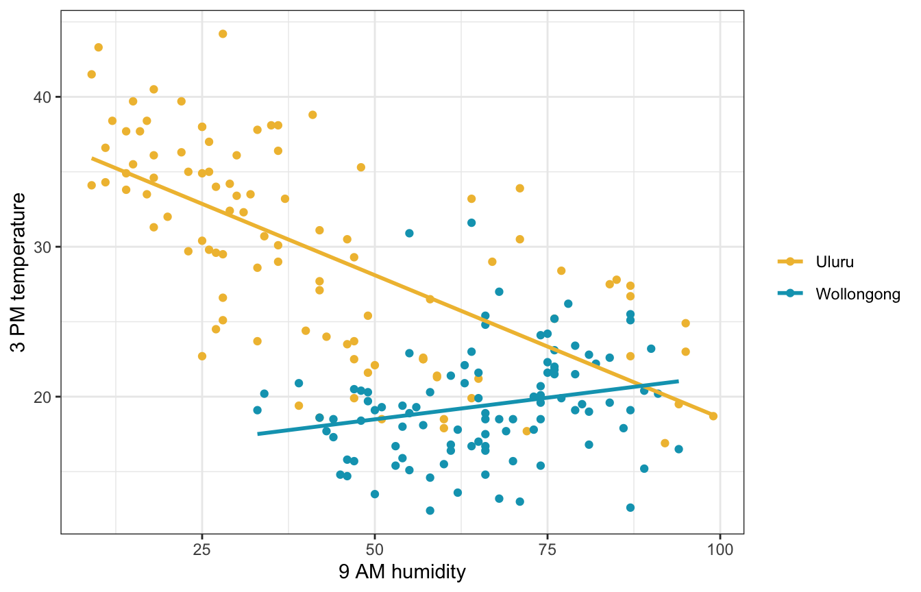
We can estimate a different slope for Wollongong by including an interaction term, which makes the model a little more complicated:
\[ \begin{aligned} Y_i \mid \beta_0, \beta_1, \beta_2, \beta_3, \sigma &\stackrel{\text{ind}}{\sim} \mathcal{N}(\mu_i, \sigma^2) \\ \mu_i &= \beta_{0c} + \beta_1 X_{i1} + \beta_2 X_{i2} + \beta_3 (X_{i1} \times X_{i2}) \\ \\ \beta_{0c} &\sim \mathcal{N}(25, 5) \\ \beta_{1} &\sim \mathcal{N}(0, 2.5) \\ \beta_{2} &\sim \mathcal{N}(0, 10) \\ \beta_{3} &\sim \mathcal{N}(0, 2.5) \\ \sigma &\sim \operatorname{Exponential}(1) \end{aligned} \]
Understanding the priors
These look fine I guess. Though only really for the autoscaled rstanarm priors. The super vague brms priors lead to some wild predictions.
weather_interaction_prior_rstanarm <- stan_glm(
  temp3pm ~ humidity9am + location + humidity9am:location,
  data = weather_WU,
  family = gaussian,
  prior_intercept = normal(25, 5),
  prior = normal(0, 2.5, autoscale = TRUE),
  prior_aux = exponential(1, autoscale = TRUE),
  chains = 4, iter = 5000*2, seed = 84735, refresh = 0,
  prior_PD = TRUE
)
p1 <- weather_WU |>
add_predicted_draws(weather_interaction_prior_rstanarm, ndraws = 100) |>
ggplot(aes(x = .prediction, group = .draw)) +
geom_density(size = 0.25, color = clrs[3]) +
labs(x = "Predicted 3 PM temperature", y = "Density")
# Feed add_epred_draws() brand new data instead of the original data, just for fun
prior_draws_rstanarm <- weather_WU |>
group_by(location) |>
summarize(min = min(humidity9am),
max = max(humidity9am)) |>
mutate(humidity9am = map2(min, max, ~seq(.x, .y, 1))) |>
unnest(humidity9am) |>
add_epred_draws(weather_interaction_prior_rstanarm, ndraws = 100)
p2 <- prior_draws_rstanarm |>
ggplot(aes(x = humidity9am, y = .epred)) +
geom_line(aes(group = paste(location, .draw), color = location), alpha = 0.2) +
scale_color_manual(values = c(clrs[2], clrs[1])) +
labs(x = "9 AM humidity", y = "3 PM temperature", color = NULL) +
theme(legend.position = "bottom")
p1 | p2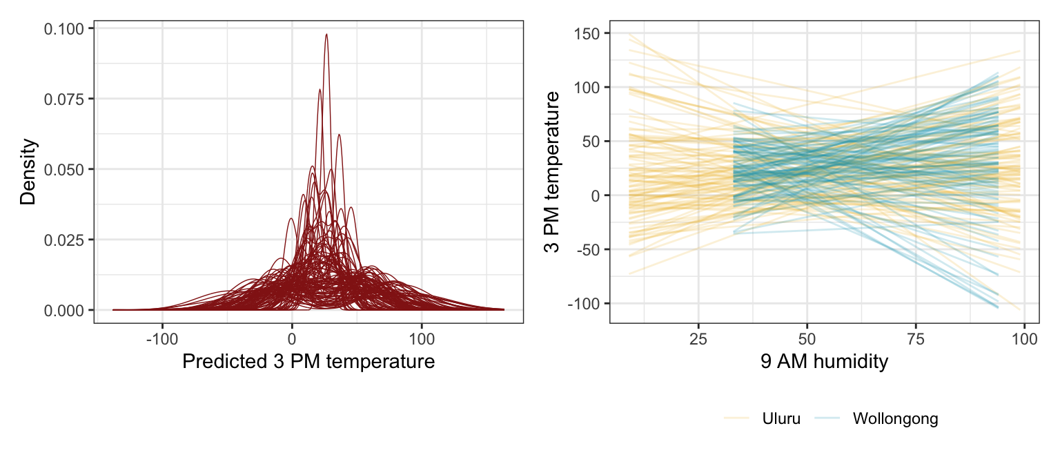
priors <- c(prior(normal(25, 5), class = Intercept),
            prior(normal(0, 2.5), class = b, coef = "humidity9am_c"),
            prior(normal(0, 10), class = b, coef = "locationWollongong"),
            prior(normal(0, 2.5), class = b, coef = "humidity9am_c:locationWollongong"),
            prior(exponential(1), class = sigma))

weather_interaction_prior_brms <- brm(
  bf(temp3pm ~ humidity9am_c + location + humidity9am_c:location),
  data = weather_WU,
  family = gaussian(),
  prior = priors,
  chains = 4, iter = 5000*2, seed = BAYES_SEED,
  backend = "cmdstanr", refresh = 0,
  sample_prior = "only"
)
## Start sampling
p1 <- weather_WU |>
add_predicted_draws(weather_interaction_prior_brms, ndraws = 100) |>
ggplot(aes(x = .prediction, group = .draw)) +
geom_density(size = 0.25, color = clrs[3]) +
labs(x = "Predicted 3 PM temperature", y = "Density")
# Feed add_epred_draws() brand new data instead of the original data, just for fun
prior_draws_brms <- weather_WU |>
group_by(location) |>
summarize(min = min(humidity9am_c),
max = max(humidity9am_c)) |>
mutate(humidity9am_c = map2(min, max, ~seq(.x, .y, 1))) |>
unnest(humidity9am_c) |>
add_epred_draws(weather_interaction_prior_brms, ndraws = 100) |>
mutate(humidity_9am = humidity9am_c + unscaled$humidity9am_centered$scaled_center)
p2 <- prior_draws_brms |>
ggplot(aes(x = humidity_9am, y = .epred)) +
geom_line(aes(group = paste(location, .draw), color = location), alpha = 0.2) +
scale_color_manual(values = c(clrs[2], clrs[1])) +
labs(x = "9 AM humidity", y = "3 PM temperature", color = NULL) +
theme(legend.position = "bottom")
p1 | p2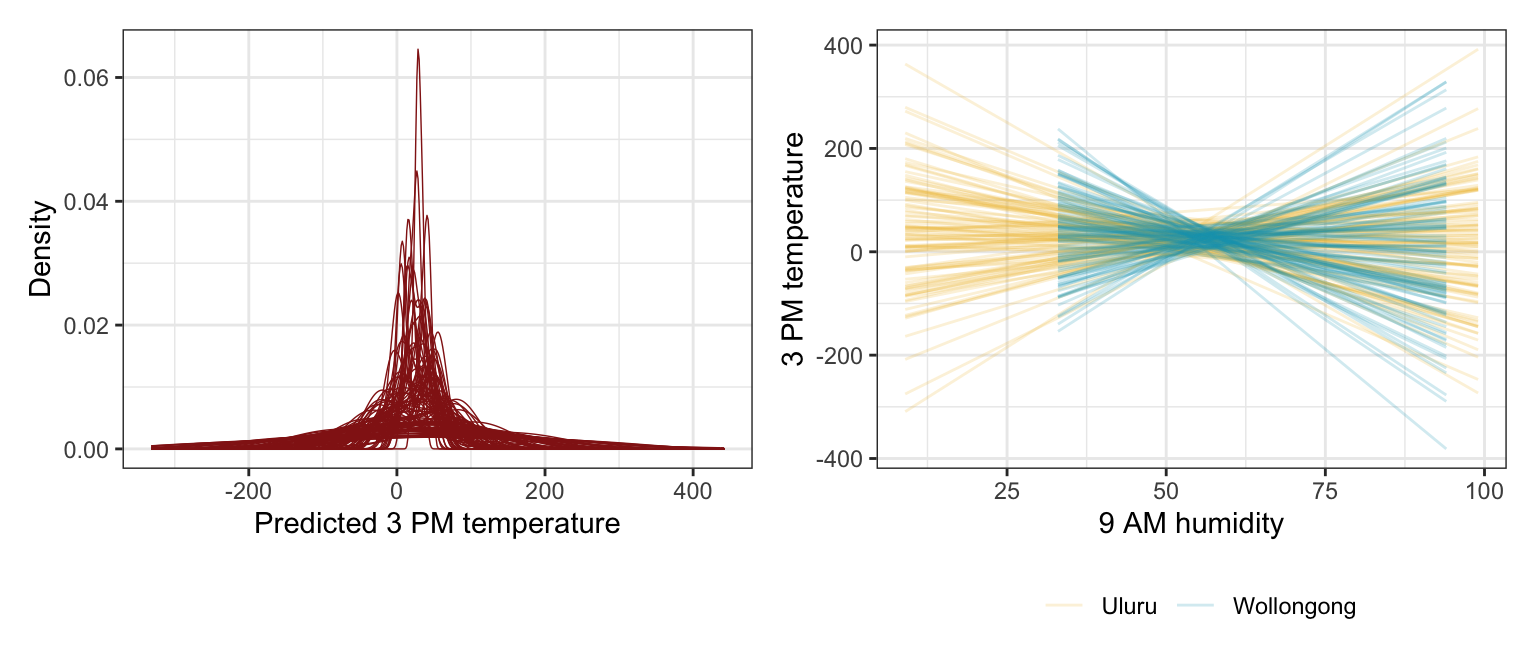
Simulating the posterior
Model
weather_interaction_rstanarm <- stan_glm(
  temp3pm ~ humidity9am + location + humidity9am:location,
  data = weather_WU,
  family = gaussian,
  prior_intercept = normal(25, 5),
  prior = normal(0, 2.5, autoscale = TRUE),
  prior_aux = exponential(1, autoscale = TRUE),
  chains = 4, iter = 5000*2, seed = 84735, refresh = 0
)tidy(weather_interaction_rstanarm, effects = c("fixed", "aux"),
conf.int = TRUE, conf.level = 0.8)
## # A tibble: 6 × 5
## term estimate std.error conf.low conf.high
## <chr> <dbl> <dbl> <dbl> <dbl>
## 1 (Intercept) 37.6 0.905 36.4 38.8
## 2 humidity9am -0.189 0.0190 -0.214 -0.165
## 3 locationWollongong -21.8 2.34 -24.8 -18.9
## 4 humidity9am:locationWollongong 0.245 0.0370 0.198 0.292
## 5 sigma 4.47 0.228 4.19 4.77
## 6 mean_PPD 24.6 0.449 24.0 25.1Coefficient posteriors
weather_interaction_rstanarm |>
  gather_draws(`(Intercept)`, humidity9am, locationWollongong, `humidity9am:locationWollongong`, sigma) |>
  ungroup() |>
  mutate(.variable = fct_relevel(factor(.variable),
                                 c("(Intercept)", "humidity9am", "locationWollongong",
                                   "humidity9am:locationWollongong", "sigma"))) |>
  ggplot(aes(x = .value, fill = .variable)) +
  stat_halfeye(normalize = "xy") +
  scale_fill_manual(values = c(clrs[1], clrs[3], clrs[4], clrs[2], clrs[5]), guide = "none") +
  facet_wrap(vars(.variable), scales = "free_x") +
  labs(x = "Parameter posterior") +
  theme(legend.position = "bottom")
## Warning: Unknown or uninitialised column: `linewidth`.
## Unknown or uninitialised column: `linewidth`.
## Unknown or uninitialised column: `linewidth`.
## Unknown or uninitialised column: `linewidth`.
## Unknown or uninitialised column: `linewidth`.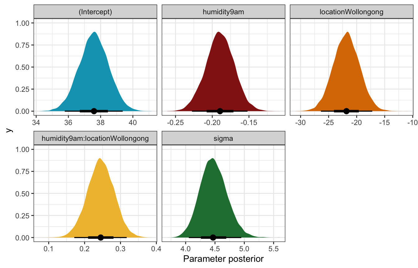
Fitted draws
weather_WU |>
  add_linpred_draws(weather_interaction_rstanarm, ndraws = 100) |>
  ggplot(aes(x = humidity9am, y = temp3pm, color = location)) +
  geom_point(data = weather_WU, size = 0.5) +
  geom_line(aes(y = .linpred, group = paste(location, .draw)), alpha = 0.2, size = 0.5) +
  scale_color_manual(values = c(clrs[2], clrs[1])) +
  labs(x = "9 AM humidity", y = "3 PM temperature", color = NULL)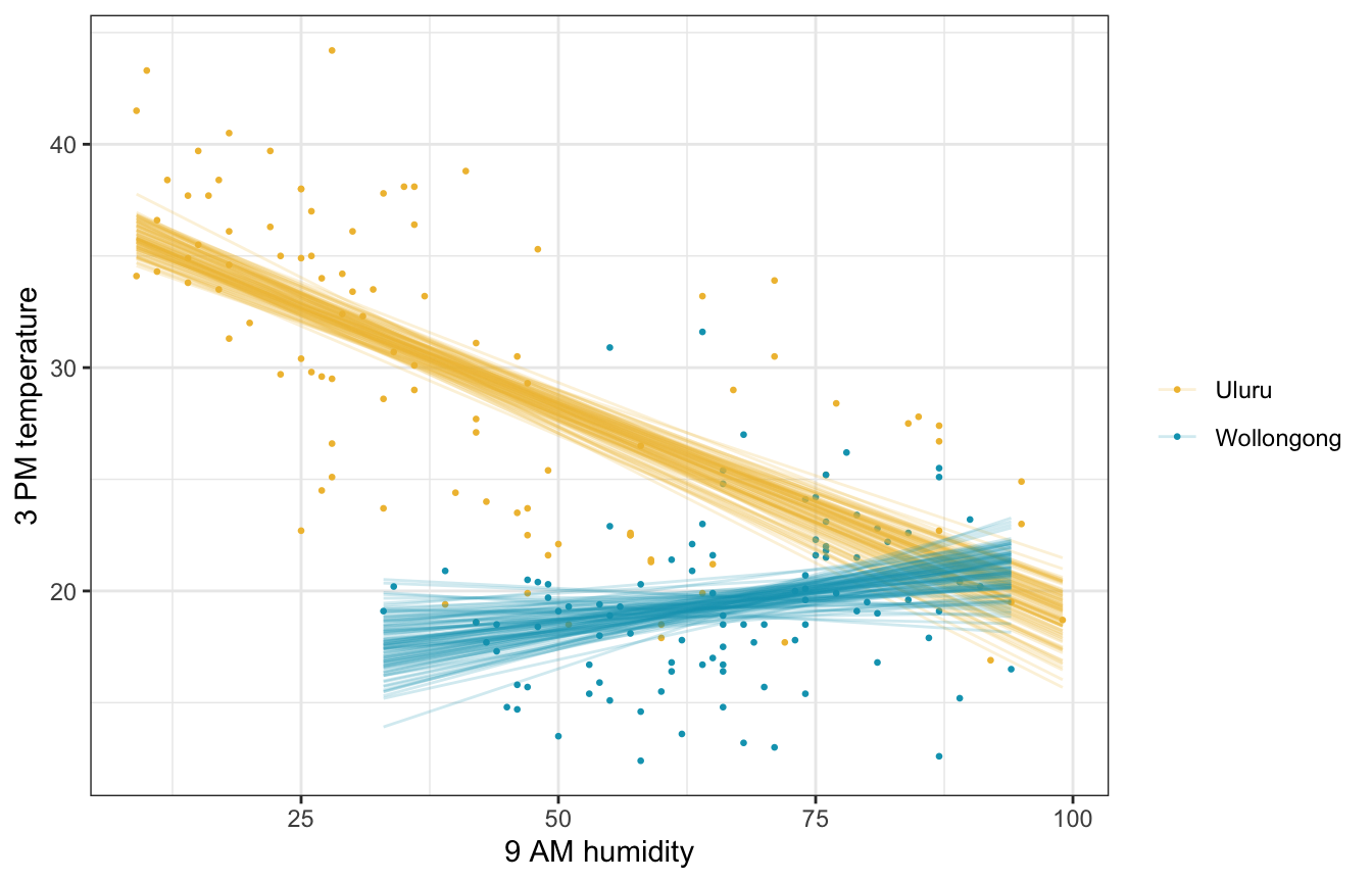
Posterior predictive check
pp_check(weather_interaction_rstanarm, n = 25)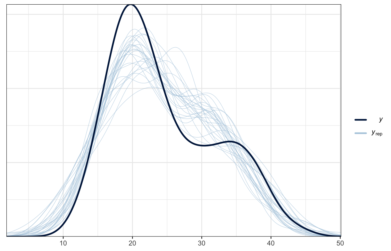
Model
priors <- c(prior(normal(25, 5), class = Intercept),
            prior(normal(0, 2.5), class = b, coef = "humidity9am_c"),
            prior(normal(0, 10), class = b, coef = "locationWollongong"),
            prior(normal(0, 2.5), class = b, coef = "humidity9am_c:locationWollongong"),
            prior(exponential(1), class = sigma))

weather_interaction_brms <- brm(
  bf(temp3pm ~ humidity9am_c + location + humidity9am_c:location),
  data = weather_WU,
  family = gaussian(),
  prior = priors,
  chains = 4, iter = 5000*2, seed = BAYES_SEED,
  backend = "cmdstanr", refresh = 0
)
## Start samplingtidy(weather_interaction_brms, conf.int = TRUE, conf.level = 0.8) |>
select(-c(effect, component, group))
## Warning in tidy.brmsfit(weather_interaction_brms, conf.int = TRUE, conf.level =
## 0.8): some parameter names contain underscores: term naming may be unreliable!
## # A tibble: 5 × 5
## term estimate std.error conf.low conf.high
## <chr> <dbl> <dbl> <dbl> <dbl>
## 1 (Intercept) 27.4 0.496 26.8 28.0
## 2 humidity9am_c -0.191 0.0190 -0.215 -0.166
## 3 locationWollongong -8.68 0.772 -9.67 -7.70
## 4 humidity9am_c:locationWollongong 0.247 0.0370 0.200 0.295
## 5 sd__Observation 4.43 0.222 4.15 4.72Coefficient posteriors
weather_interaction_brms |>
  gather_draws(b_Intercept, b_humidity9am_c, b_locationWollongong,
               `b_humidity9am_c:locationWollongong`, sigma) |>
  ungroup() |>
  mutate(.variable = fct_relevel(factor(.variable),
                                 c("b_Intercept", "b_humidity9am_c", "b_locationWollongong",
                                   "b_humidity9am_c:locationWollongong", "sigma"))) |>
  ggplot(aes(x = .value, fill = .variable)) +
  stat_halfeye(normalize = "xy") +
  scale_fill_manual(values = c(clrs[1], clrs[3], clrs[4], clrs[2], clrs[5]), guide = "none") +
  facet_wrap(vars(.variable), scales = "free_x") +
  labs(x = "Parameter posterior") +
  theme(legend.position = "bottom")
## Warning: Unknown or uninitialised column: `linewidth`.
## Unknown or uninitialised column: `linewidth`.
## Unknown or uninitialised column: `linewidth`.
## Unknown or uninitialised column: `linewidth`.
## Unknown or uninitialised column: `linewidth`.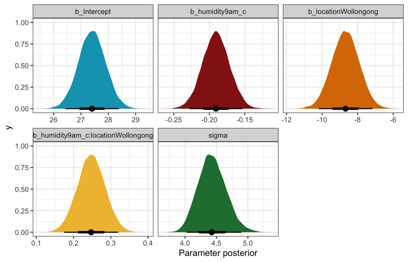
Fitted draws
weather_WU |>
  add_linpred_draws(weather_interaction_brms, ndraws = 100) |>
  ggplot(aes(x = humidity9am, y = temp3pm, color = location)) +
  geom_point(data = weather_WU, size = 0.5) +
  geom_line(aes(y = .linpred, group = paste(location, .draw)), alpha = 0.2, size = 0.5) +
  scale_color_manual(values = c(clrs[2], clrs[1])) +
  labs(x = "9 AM humidity", y = "3 PM temperature", color = NULL)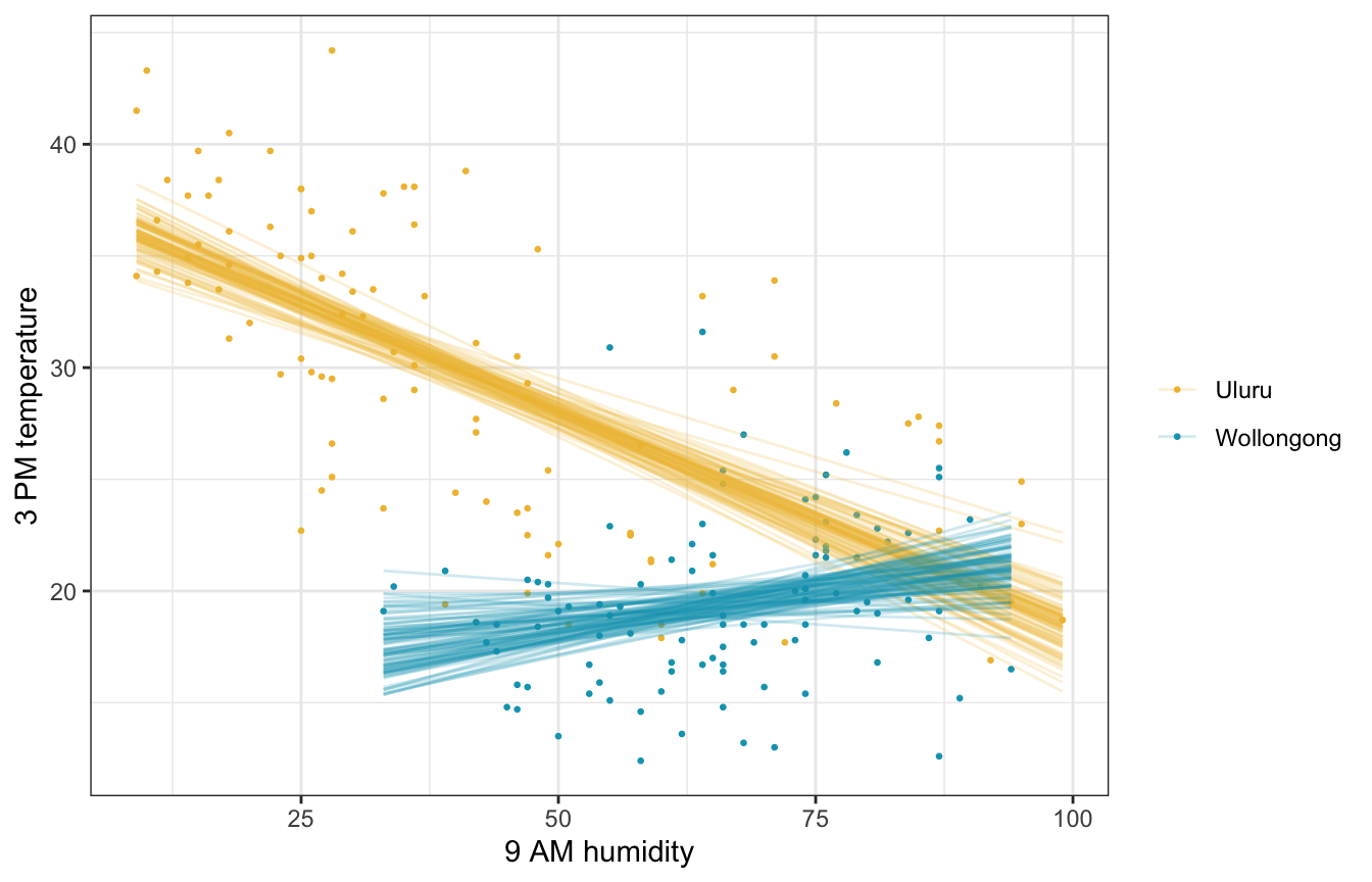
Posterior predictive check
pp_check(weather_interaction_brms, ndraws = 25)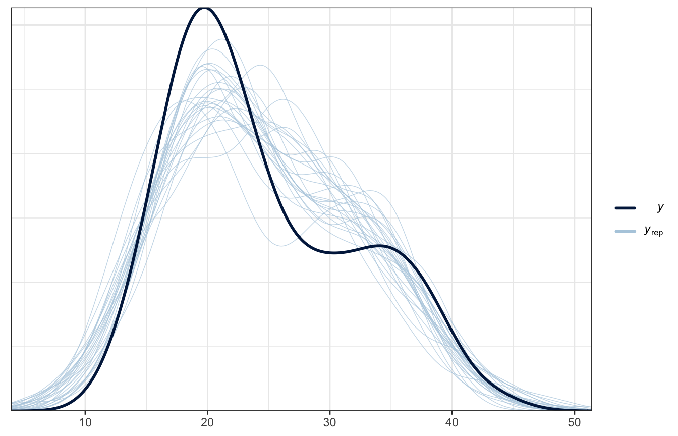
Posterior prediction
What if there’s 50% humidity at 9 AM in both cities? What’s the predicted afternoon temperature?
weather_interaction_rstanarm |>
  predicted_draws(newdata = expand_grid(humidity9am = 50,
                                        location = c("Wollongong", "Uluru"))) |>
  ggplot(aes(x = .prediction, y = location, fill = location)) +
  stat_halfeye() +
  scale_fill_manual(values = c(clrs[2], clrs[1]), guide = "none") +
  labs(x = "Predicted 3 PM temperature", y = NULL)
weather_interaction_brms |>
  predicted_draws(newdata = expand_grid(humidity9am_c = 50 - unscaled$humidity9am_centered$scaled_center,
                                        location = c("Wollongong", "Uluru"))) |>
  ggplot(aes(x = .prediction, y = location, fill = location)) +
  stat_halfeye() +
  scale_fill_manual(values = c(clrs[2], clrs[1]), guide = "none") +
  labs(x = "Predicted 3 PM temperature", y = NULL)
11.4: Utilizing more than 2 predictors
Let’s go wild and use everything!
\[ \begin{aligned} Y_i \mid \beta_0, \beta_1, \beta_2, \beta_3, \beta_4, \beta_5, \sigma &\stackrel{\text{ind}}{\sim} \mathcal{N}(\mu_i, \sigma^2) \\ \mu_i &= \beta_{0c} + \beta_1 X_{i1} + \beta_2 X_{i2} + \beta_3 X_{i3} + \beta_4 X_{i4} + \beta_5 X_{i5}\\ \\ \beta_{0c} &\sim \mathcal{N}(25, 5) \\ \beta_{1} \dots \beta_5 &\sim \mathcal{N}(0, 2.5) \\ \sigma &\sim \operatorname{Exponential}(1) \end{aligned} \]
Understanding the priors
These look fine to me. brms priors could be better, but whatever.
weather_full_prior_rstanarm <- stan_glm(
  temp3pm ~ temp9am + humidity9am + windspeed9am + pressure9am + location,
  data = weather_WU,
  family = gaussian,
  prior_intercept = normal(25, 5),
  prior = normal(0, 2.5, autoscale = TRUE),
  prior_aux = exponential(1, autoscale = TRUE),
  chains = 4, iter = 5000*2, seed = 84735, refresh = 0,
  prior_PD = TRUE
)
weather_WU |>
add_predicted_draws(weather_full_prior_rstanarm, ndraws = 100) |>
ggplot(aes(x = .prediction, group = .draw)) +
geom_density(size = 0.25, color = clrs[3]) +
labs(x = "Predicted 3 PM temperature", y = "Density")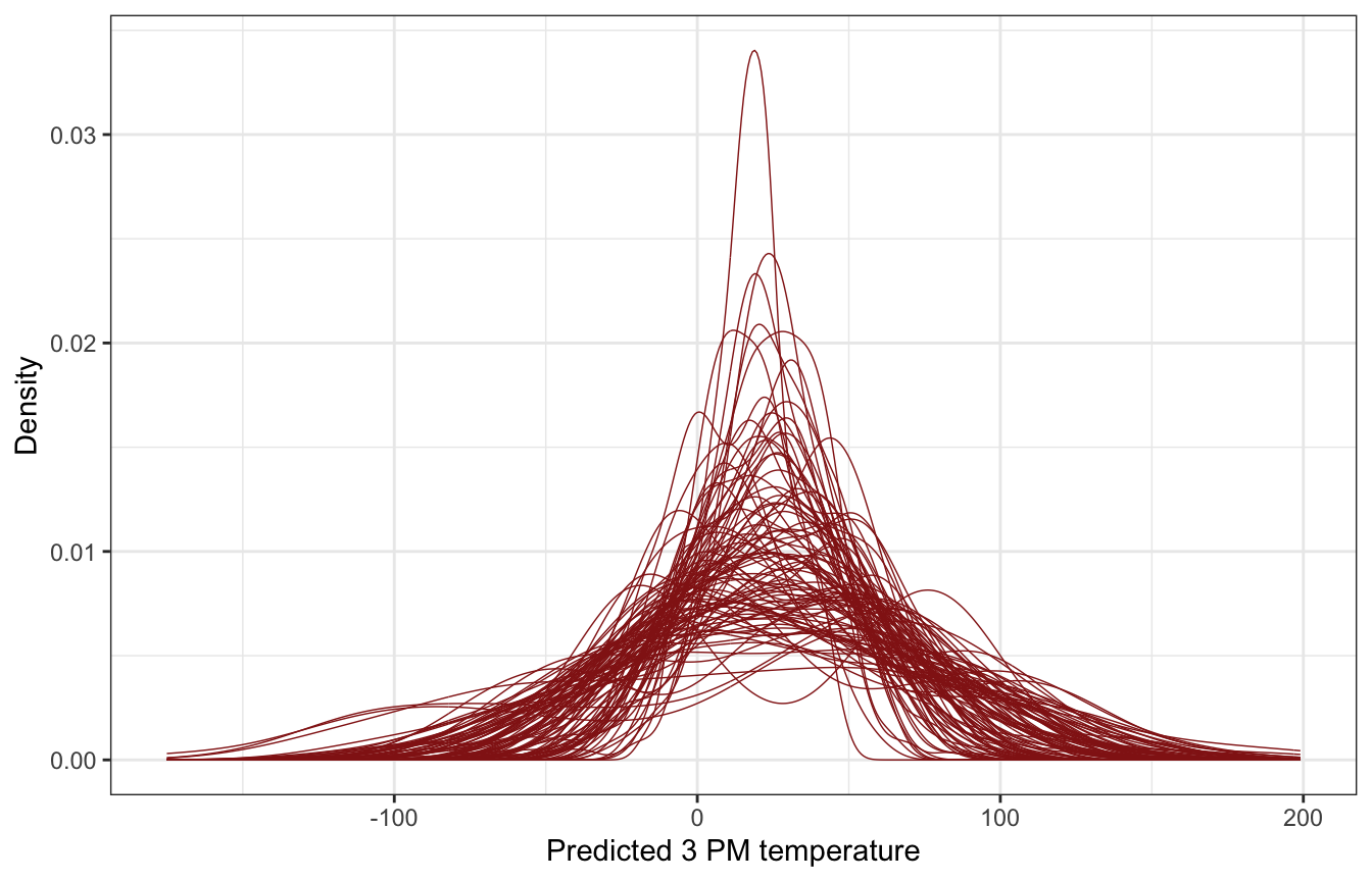
priors <- c(prior(normal(25, 5), class = Intercept),
            prior(normal(0, 2.5), class = b),
            prior(exponential(1), class = sigma))

weather_full_prior_brms <- brm(
  bf(temp3pm ~ temp9am_c + humidity9am_c + windspeed9am_c + pressure9am_c + location),
  data = weather_WU,
  family = gaussian(),
  prior = priors,
  chains = 4, iter = 5000*2, seed = BAYES_SEED,
  backend = "cmdstanr", refresh = 0,
  sample_prior = "only"
)
## Start sampling
weather_WU |>
add_predicted_draws(weather_full_prior_brms, ndraws = 100) |>
ggplot(aes(x = .prediction, group = .draw)) +
geom_density(size = 0.25, color = clrs[3]) +
labs(x = "Predicted 3 PM temperature", y = "Density")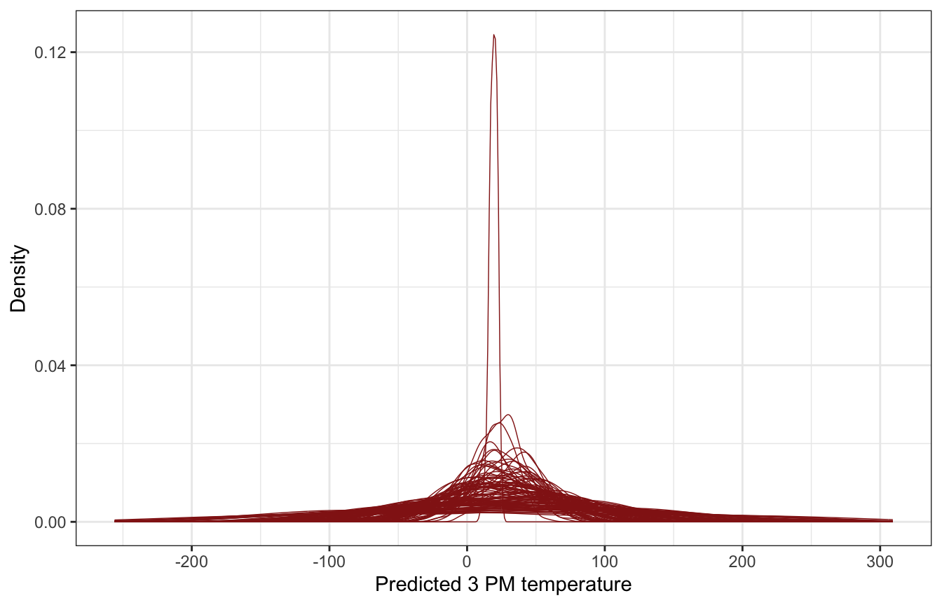
Simulating the posterior
Model
weather_full_rstanarm <- stan_glm(
  temp3pm ~ temp9am + humidity9am + windspeed9am + pressure9am + location,
  data = weather_WU,
  family = gaussian,
  prior_intercept = normal(25, 5),
  prior = normal(0, 2.5, autoscale = TRUE),
  prior_aux = exponential(1, autoscale = TRUE),
  chains = 4, iter = 5000*2, seed = 84735, refresh = 0
)tidy(weather_full_rstanarm, effects = c("fixed", "aux"),
conf.int = TRUE, conf.level = 0.8)
## # A tibble: 8 × 5
## term estimate std.error conf.low conf.high
## <chr> <dbl> <dbl> <dbl> <dbl>
## 1 (Intercept) 37.6 30.8 -2.07 76.8
## 2 temp9am 0.802 0.0366 0.756 0.850
## 3 humidity9am -0.0338 0.00927 -0.0458 -0.0218
## 4 windspeed9am -0.0131 0.0211 -0.0398 0.0142
## 5 pressure9am -0.0231 0.0299 -0.0610 0.0154
## 6 locationWollongong -6.42 0.388 -6.92 -5.92
## 7 sigma 2.32 0.120 2.17 2.48
## 8 mean_PPD 24.6 0.233 24.3 24.9Coefficient posteriors
weather_full_rstanarm |>
  gather_draws(`(Intercept)`, temp9am, humidity9am, windspeed9am,
               pressure9am, locationWollongong, sigma) |>
  ungroup() |>
  mutate(.variable = fct_relevel(factor(.variable),
                                 c("(Intercept)", "temp9am", "humidity9am", "windspeed9am",
                                   "pressure9am", "locationWollongong", "sigma"))) |>
  ggplot(aes(x = .value, fill = .variable)) +
  stat_halfeye(normalize = "xy") +
  guides(fill = "none") +
  facet_wrap(vars(.variable), scales = "free_x") +
  labs(x = "Parameter posterior") +
  theme(legend.position = "bottom")
## Warning: Unknown or uninitialised column: `linewidth`.
## Unknown or uninitialised column: `linewidth`.
## Unknown or uninitialised column: `linewidth`.
## Unknown or uninitialised column: `linewidth`.
## Unknown or uninitialised column: `linewidth`.
## Unknown or uninitialised column: `linewidth`.
## Unknown or uninitialised column: `linewidth`.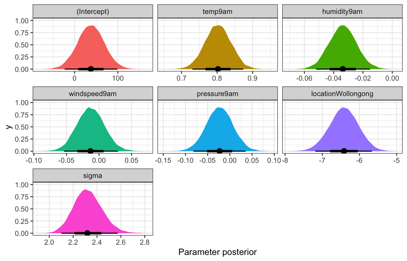
Posterior predictive check
Super nice now
pp_check(weather_full_rstanarm, n = 25)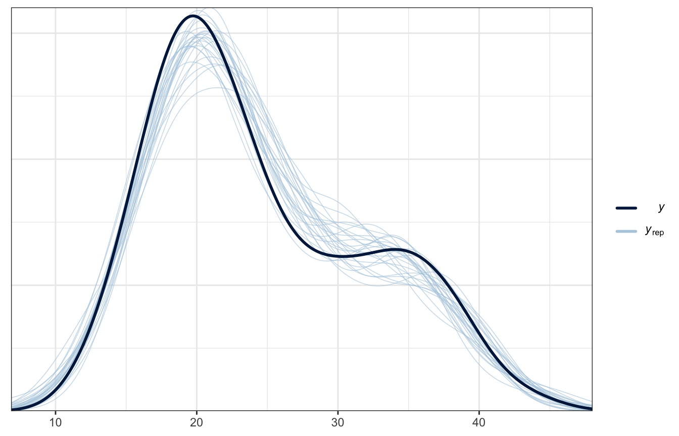
Model
priors <- c(prior(normal(25, 5), class = Intercept),
            prior(normal(0, 2.5), class = b),
            prior(exponential(1), class = sigma))

weather_full_brms <- brm(
  bf(temp3pm ~ temp9am_c + humidity9am_c + windspeed9am_c + pressure9am_c + location),
  data = weather_WU,
  family = gaussian(),
  prior = priors,
  chains = 4, iter = 5000*2, seed = BAYES_SEED,
  backend = "cmdstanr", refresh = 0
)
## Start samplingtidy(weather_full_brms, conf.int = TRUE, conf.level = 0.8) |>
select(-c(effect, component, group))
## Warning in tidy.brmsfit(weather_full_brms, conf.int = TRUE, conf.level = 0.8):
## some parameter names contain underscores: term naming may be unreliable!
## # A tibble: 7 × 5
## term estimate std.error conf.low conf.high
## <chr> <dbl> <dbl> <dbl> <dbl>
## 1 (Intercept) 27.7 0.255 27.4 28.0
## 2 temp9am_c 0.804 0.0364 0.758 0.850
## 3 humidity9am_c -0.0354 0.00919 -0.0471 -0.0237
## 4 windspeed9am_c -0.0138 0.0213 -0.0412 0.0136
## 5 pressure9am_c -0.0221 0.0299 -0.0604 0.0166
## 6 locationWollongong -6.27 0.387 -6.77 -5.77
## 7 sd__Observation 2.31 0.117 2.17 2.47Coefficient posteriors
get_variables(weather_full_brms)
##  [1] "b_Intercept"          "b_temp9am_c"          "b_humidity9am_c"
##  [4] "b_windspeed9am_c"     "b_pressure9am_c"      "b_locationWollongong"
##  [7] "sigma"                "lprior"               "lp__"
## [10] "accept_stat__"        "treedepth__"          "stepsize__"
## [13] "divergent__"          "n_leapfrog__"         "energy__"
weather_full_brms |>
  gather_draws(b_Intercept, b_temp9am_c, b_humidity9am_c, b_windspeed9am_c,
               b_pressure9am_c, b_locationWollongong, sigma) |>
  ungroup() |>
  mutate(.variable = fct_relevel(factor(.variable),
                                 c("b_Intercept", "b_temp9am_c", "b_humidity9am_c", "b_windspeed9am_c",
                                   "b_pressure9am_c", "b_locationWollongong", "sigma"))) |>
  ggplot(aes(x = .value, fill = .variable)) +
  stat_halfeye(normalize = "xy") +
  guides(fill = "none") +
  facet_wrap(vars(.variable), scales = "free_x") +
  labs(x = "Parameter posterior") +
  theme(legend.position = "bottom")
## Warning: Unknown or uninitialised column: `linewidth`.
## Unknown or uninitialised column: `linewidth`.
## Unknown or uninitialised column: `linewidth`.
## Unknown or uninitialised column: `linewidth`.
## Unknown or uninitialised column: `linewidth`.
## Unknown or uninitialised column: `linewidth`.
## Unknown or uninitialised column: `linewidth`.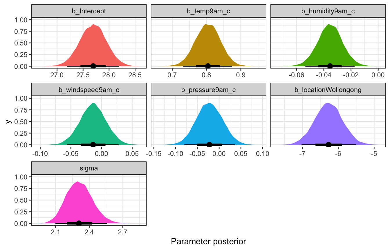
Posterior predictive check
Delightful.
pp_check(weather_full_brms, ndraws = 25)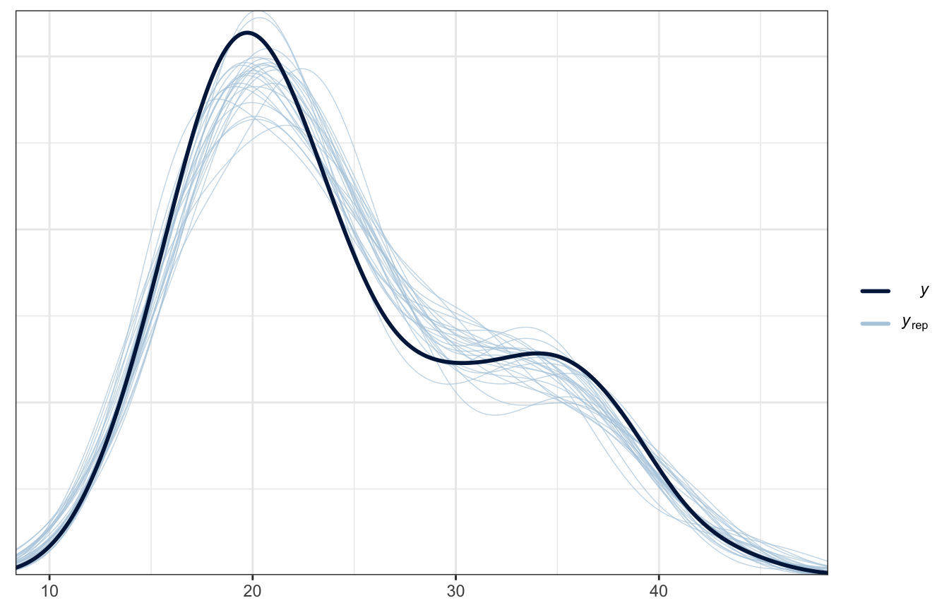
Posterior prediction
What if there’s 50% humidity, 10 MPH of wind, pressure of 1015, and temperature of 10˚ at 9 AM in both cities? What’s the predicted afternoon temperature?
weather_full_rstanarm |>
  predicted_draws(newdata = expand_grid(humidity9am = 50,
                                        windspeed9am = 10,
                                        pressure9am = 1015,
                                        temp9am = 10,
                                        location = c("Wollongong", "Uluru"))) |>
  ggplot(aes(x = .prediction, y = location, fill = location)) +
  stat_halfeye() +
  scale_fill_manual(values = c(clrs[2], clrs[1]), guide = "none") +
  labs(x = "Predicted 3 PM temperature", y = NULL)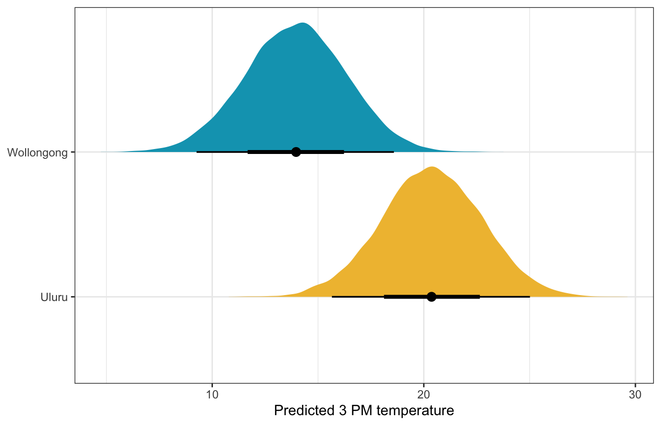
weather_full_brms |>
  predicted_draws(newdata = expand_grid(humidity9am_c = 50 - unscaled$humidity9am_centered$scaled_center,
                                        windspeed9am_c = 10 - unscaled$windspeed9am_centered$scaled_center,
                                        pressure9am_c = 1015 - unscaled$pressure9am_centered$scaled_center,
                                        temp9am_c = 10 - unscaled$temp9am_centered$scaled_center,
                                        location = c("Wollongong", "Uluru"))) |>
  ggplot(aes(x = .prediction, y = location, fill = location)) +
  stat_halfeye() +
  scale_fill_manual(values = c(clrs[2], clrs[1]), guide = "none") +
  labs(x = "Predicted 3 PM temperature", y = NULL)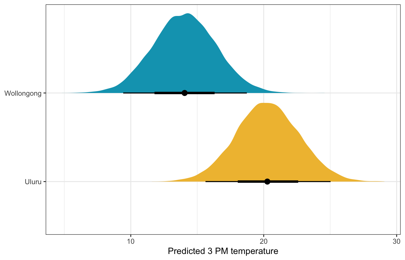
11.5: Model evaluation and comparison
Phew. We have 5 (actually 10) different models predicting afternoon temperature:
weather_simple_rstanarm and weather_simple_brms |
|
|
weather_location_only_rstanarm and weather_location_only_brms |
|
|
weather_location_rstanarm and weather_location_brms |
|
|
weather_interaction_rstanarm and weather_interaction_brms |
|
|
weather_full_rstanarm and weather_full_brms |
|
|
How fair is each model?
That’s fine here. They’re all equally fair (and the data was collected through an automated system and seems fair)
How wrong is each model?
We can compare all the posterior predictive checks. y_rep gets better as the model gets more complex.
models_rstanarm <- tribble(
  ~model_name, ~model,
  "Temperature only", weather_simple_rstanarm,
  "Location only", weather_location_only_rstanarm,
  "Temperature + location", weather_location_rstanarm,
  "Temperature × location", weather_interaction_rstanarm,
  "Full model", weather_full_rstanarm
) |>
  mutate(ppcheck = map2(model, model_name, ~pp_check(.x, n = 25) + labs(title = .y))) |>
mutate(loo = map(model, ~loo(.)))wrap_plots(models_rstanarm$ppcheck)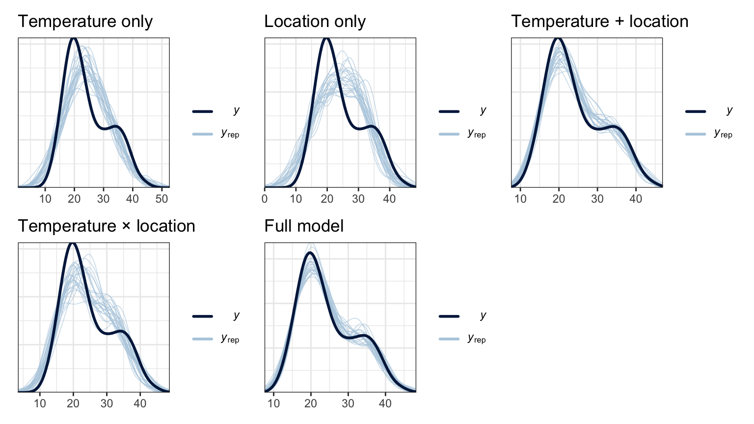
models_brms <- tribble(
  ~model_name, ~model,
  "Temperature only", weather_simple_brms,
  "Location only", weather_location_only_brms,
  "Temperature + location", weather_location_brms,
  "Temperature × location", weather_interaction_brms,
  "Full model", weather_full_brms
) |>
  mutate(ppcheck = map2(model, model_name, ~pp_check(.x, ndraws = 25) + labs(title = .y))) |>
mutate(loo = map(model, ~loo(.)))wrap_plots(models_brms$ppcheck)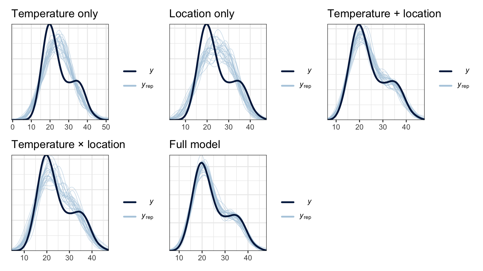
How accurate are each model’s predictions?
We can check these with the 3 approaches from chapter 10.
Visualization
For the models with fewer dimensions we can visualize their predictions, like with the location-only model and the model with the interaction
weather_location_only_rstanarm |>
  add_predicted_draws(newdata = weather_WU, ndraws = 100) |>
  ggplot(aes(x = location)) +
  stat_dotsinterval(aes(y = .prediction, color = location, fill = location),
                    quantiles = 300, side = "right", slab_size = 0, scale = 0.4) +
  stat_dotsinterval(aes(y = temp3pm, fill = location),
                    side = "left", quantiles = 100, slab_size = 0, slab_shape = 23) +
  scale_fill_manual(values = c(clrs[2], clrs[1]), guide = "none") +
  guides(color = "none") +
  labs(title = "Actual data on left; predictions on right",
       y = "Predicted afternoon temperature", x = NULL)
weather_location_only_brms |>
  add_predicted_draws(newdata = weather_WU, ndraws = 100) |>
  ggplot(aes(x = location)) +
  stat_dotsinterval(aes(y = .prediction, color = location, fill = location),
                    quantiles = 300, side = "right", slab_size = 0, scale = 0.4) +
  stat_dotsinterval(aes(y = temp3pm, fill = location),
                    side = "left", quantiles = 100, slab_size = 0, slab_shape = 23) +
  scale_fill_manual(values = c(clrs[2], clrs[1]), guide = "none") +
  guides(color = "none") +
  labs(title = "Actual data on left; predictions on right",
       y = "Predicted afternoon temperature", x = NULL)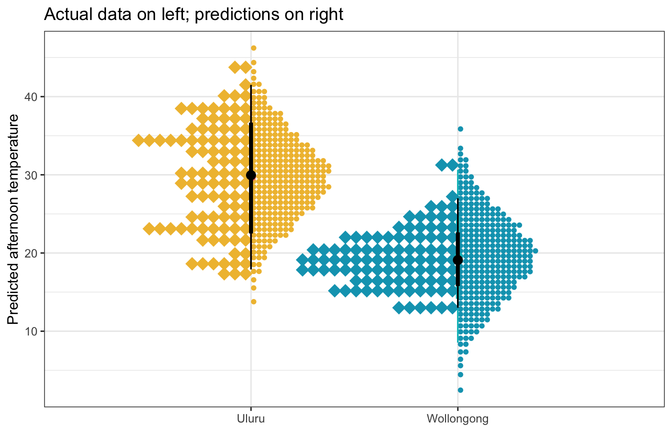
weather_interaction_rstanarm |>
  add_predicted_draws(newdata = weather_WU, ndraws = 100) |>
  ggplot(aes(x = temp9am)) +
  stat_interval(aes(y = .prediction, color = location, color_ramp = stat(level)), alpha = 0.25,
                .width = c(0.5, 0.89, 0.95)) +
  geom_point(aes(y = temp3pm, fill = location), size = 2, pch = 21, color = "white") +
  scale_color_manual(values = c(clrs[2], clrs[1])) +
  scale_fill_manual(values = c(clrs[2], clrs[1]))
## Warning: `stat(level)` was deprecated in ggplot2 3.4.0.
## ℹ Please use `after_stat(level)` instead.
weather_interaction_brms |>
  add_predicted_draws(newdata = weather_WU, ndraws = 100) |>
  ggplot(aes(x = temp9am)) +
  stat_interval(aes(y = .prediction, color = location, color_ramp = stat(level)), alpha = 0.25,
                .width = c(0.5, 0.89, 0.95)) +
  geom_point(aes(y = temp3pm, fill = location), size = 2, pch = 21, color = "white") +
  scale_color_manual(values = c(clrs[2], clrs[1])) +
  scale_fill_manual(values = c(clrs[2], clrs[1]))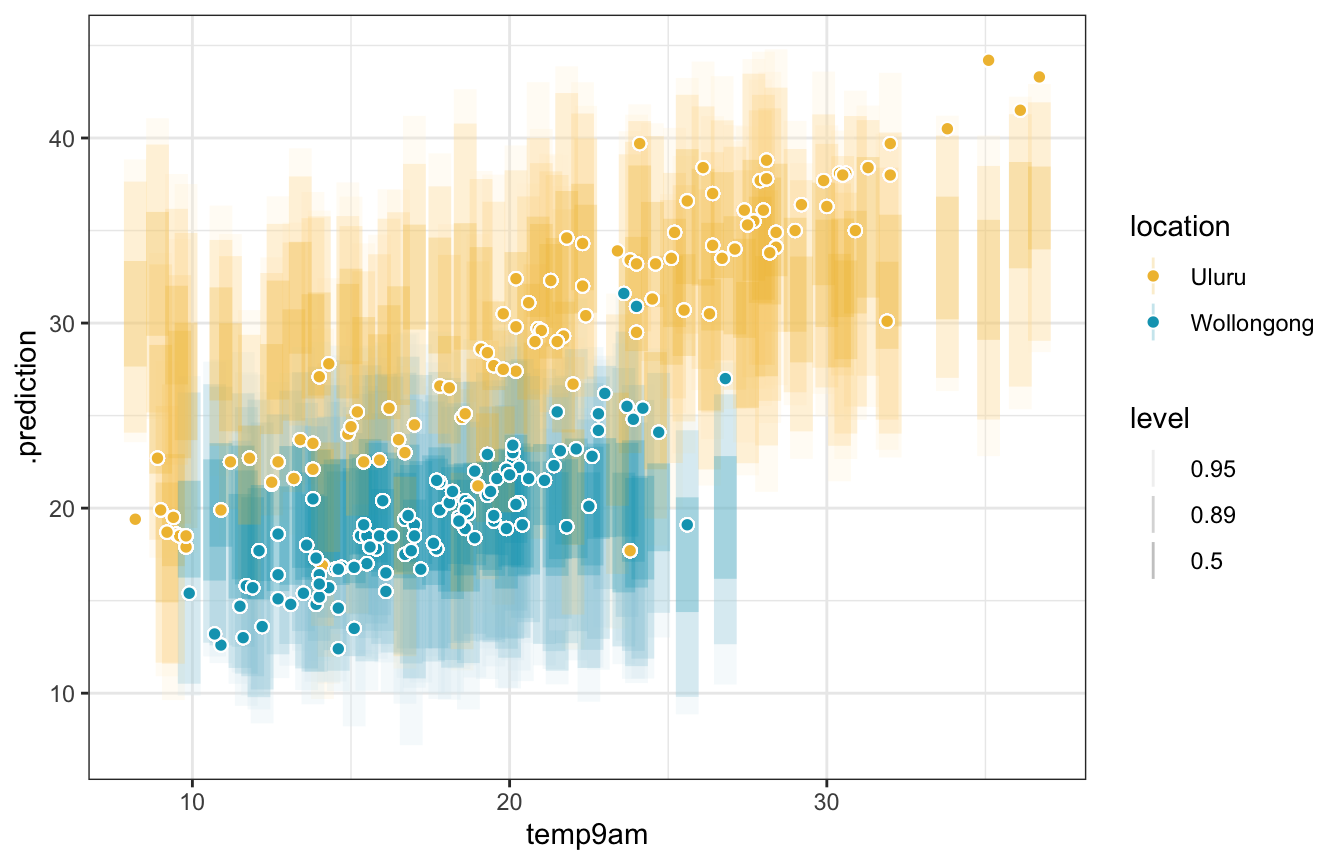
We can’t visualize the predictions from the full model without holding a bunch of stuff constant, though. So we use numbers instead!
Cross validation
We could run k-fold cross validation here, but we’d need to run 100 different Stan models (10 folds for each of the 10 models) and I don’t want to do that. The book has results from the rstanarm models. It shows that the smaller temp9am + location model is the most efficient of the bunch.
ELPD
The full model and temperature + location models have the highest ELPD, but they’re not significantly different from each other, so they perform about the same. The Bayes Rules! authors conclude:
Again, since [the temperature + location model] is simpler and achieves similar predictive accuracy, we’d personally choose to use it over the more complicated [full model].
loo_rstanarm <- models_rstanarm |>
  mutate(loo_stuff = map(loo, ~as_tibble(.$estimates, rownames = "statistic"))) |>
  select(model_name, loo_stuff) |>
  unnest(loo_stuff) |>
  filter(statistic == "elpd_loo") |>
  arrange(desc(Estimate))
loo_rstanarm
## # A tibble: 5 × 4
##   model_name             statistic Estimate    SE
##   <chr>                  <chr>        <dbl> <dbl>
## 1 Full model             elpd_loo     -458. 22.0
## 2 Temperature + location elpd_loo     -461. 23.0
## 3 Temperature only       elpd_loo     -568.  8.57
## 4 Temperature × location elpd_loo     -585.  9.99
## 5 Location only          elpd_loo     -626.  9.52
loo_rstanarm |>
mutate(model_name = fct_rev(fct_inorder(model_name))) |>
ggplot(aes(x = Estimate, y = model_name)) +
geom_pointrange(aes(xmin = Estimate - 2 * SE, xmax = Estimate + 2 * SE))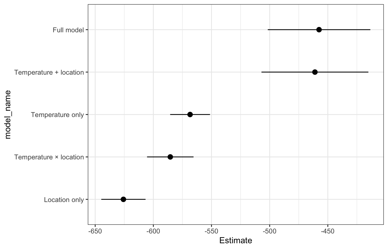
models_rstanarm |>
  pull(loo) |>
  set_names(models_rstanarm$model_name) |>
  loo_compare()
##                        elpd_diff se_diff
## Full model                0.0       0.0
## Temperature + location   -3.6       4.0
## Temperature only       -110.9      18.1
## Temperature × location -127.9      22.7
## Location only          -168.2      21.5
loo_brms <- models_brms |>
mutate(loo_stuff = map(loo, ~as_tibble(.$estimates, rownames = "statistic"))) |>
select(model_name, loo_stuff) |>
unnest(loo_stuff) |>
filter(statistic == "elpd_loo") |>
arrange(desc(Estimate))
loo_brms
## # A tibble: 5 × 4
## model_name statistic Estimate SE
## <chr> <chr> <dbl> <dbl>
## 1 Full model elpd_loo -458. 22.0
## 2 Temperature + location elpd_loo -461. 23.2
## 3 Temperature only elpd_loo -568. 8.74
## 4 Temperature × location elpd_loo -585. 10.2
## 5 Location only elpd_loo -626. 9.71loo_brms |>
mutate(model_name = fct_rev(fct_inorder(model_name))) |>
ggplot(aes(x = Estimate, y = model_name)) +
geom_pointrange(aes(xmin = Estimate - 2 * SE, xmax = Estimate + 2 * SE))
models_brms |>
  pull(loo) |>
  set_names(models_brms$model_name) |>
  loo_compare()
##                        elpd_diff se_diff
## Full model                0.0       0.0
## Temperature + location   -3.6       4.4
## Temperature only       -110.9      17.9
## Temperature × location -127.9      22.7
## Location only          -168.2      21.6