3: The Beta-Binomial Bayesian Model

Reading notes

library(bayesrules)
library(tidyverse)
library(extraDistr)
library(brms)
library(tidybayes)

# Plot stuff
clrs <- MetBrewer::met.brewer("Lakota", 6)
theme_set(theme_bw())

# Seed stuff
BAYES_SEED <- 1234
set.seed(1234)

3.1: Beta prior model

\[ \pi \sim \operatorname{Beta}(45, 55) \]

ggplot() +
  geom_function(fun = ~dbeta(., 45, 55), n = 1001) +
  labs(title = "dbeta(45, 55)")

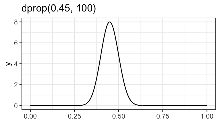
ggplot() +
  geom_function(fun = ~dprop(., mean = 0.45, size = 100), n = 1001) +
  labs(title = "dprop(0.45, 100)")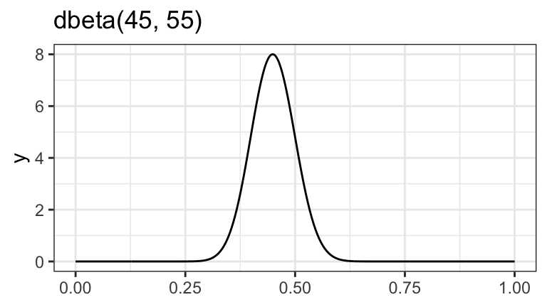

3.2: Binomial data model and likelihood

\[ Y \mid \pi = \operatorname{Binomial}(50, \pi) \]

3.3: Beta posterior model

\[ \begin{aligned} Y \mid \pi &= \operatorname{Binomial}(50, \pi) \\ \pi &\sim \operatorname{Beta}(45, 55) \end{aligned} \]

model_election <- brm(
  bf(support | trials(n_in_poll) ~ 0 + Intercept),
  data = list(support = 30, n_in_poll = 50),
  family = binomial(link = "identity"),
  prior(beta(45, 55), class = b, lb = 0, ub = 1),
  iter = 5000, warmup = 1000, seed = BAYES_SEED,
  backend = "rstan", cores = 4
)
## Compiling Stan program...
## Start sampling

model_election %>% 
  gather_draws(b_Intercept) %>% 
  ggplot(aes(x = .value)) +
  stat_halfeye(fill = clrs[6]) +
  labs(x = "π", title = "Plausible values of π that could produce\na poll where 30/50 voters support Michelle")
## Warning: Using the `size` aesthietic with geom_segment was deprecated in ggplot2 3.4.0.
## ℹ Please use the `linewidth` aesthetic instead.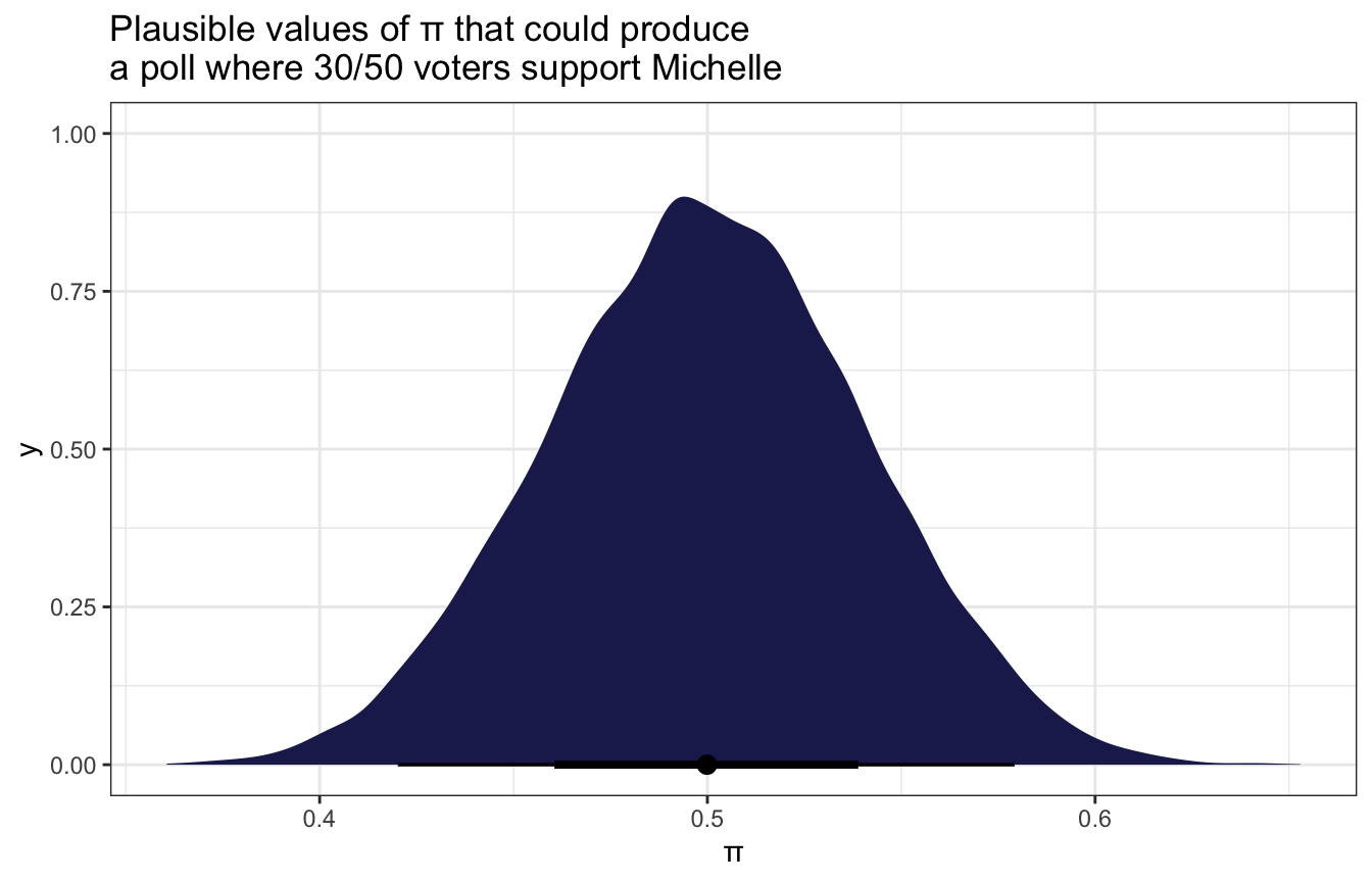

model_election %>% 
  gather_draws(b_Intercept) %>% 
  ggplot(aes(x = .value)) +
  geom_density(aes(fill = "Posterior"), color = NA, alpha = 0.75) +
  stat_function(geom = "area", fun = ~dbeta(., 45, 55), aes(fill = "Beta(45, 55) prior"), alpha = 0.75) +
  scale_fill_manual(values = clrs[5:6])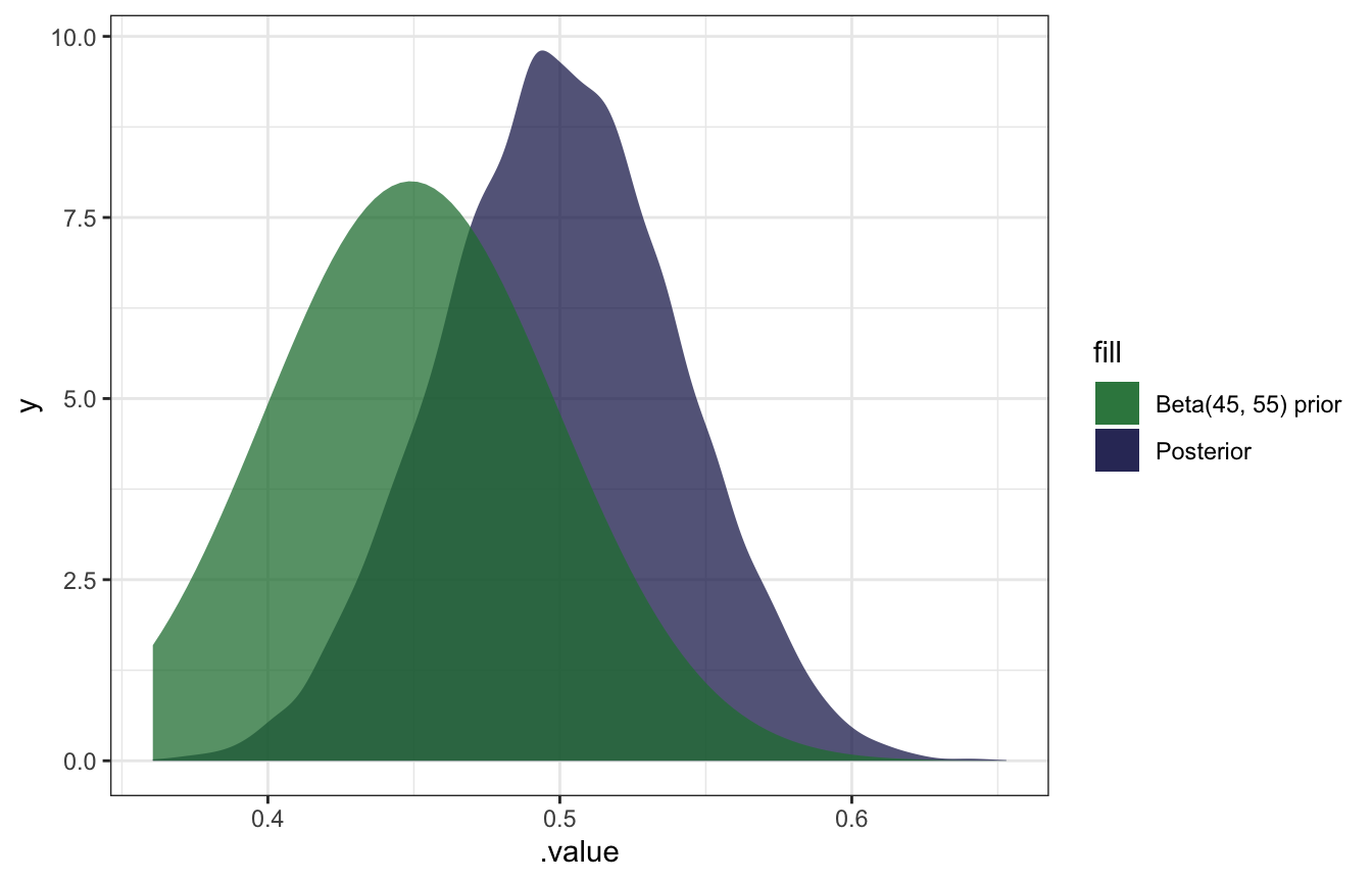

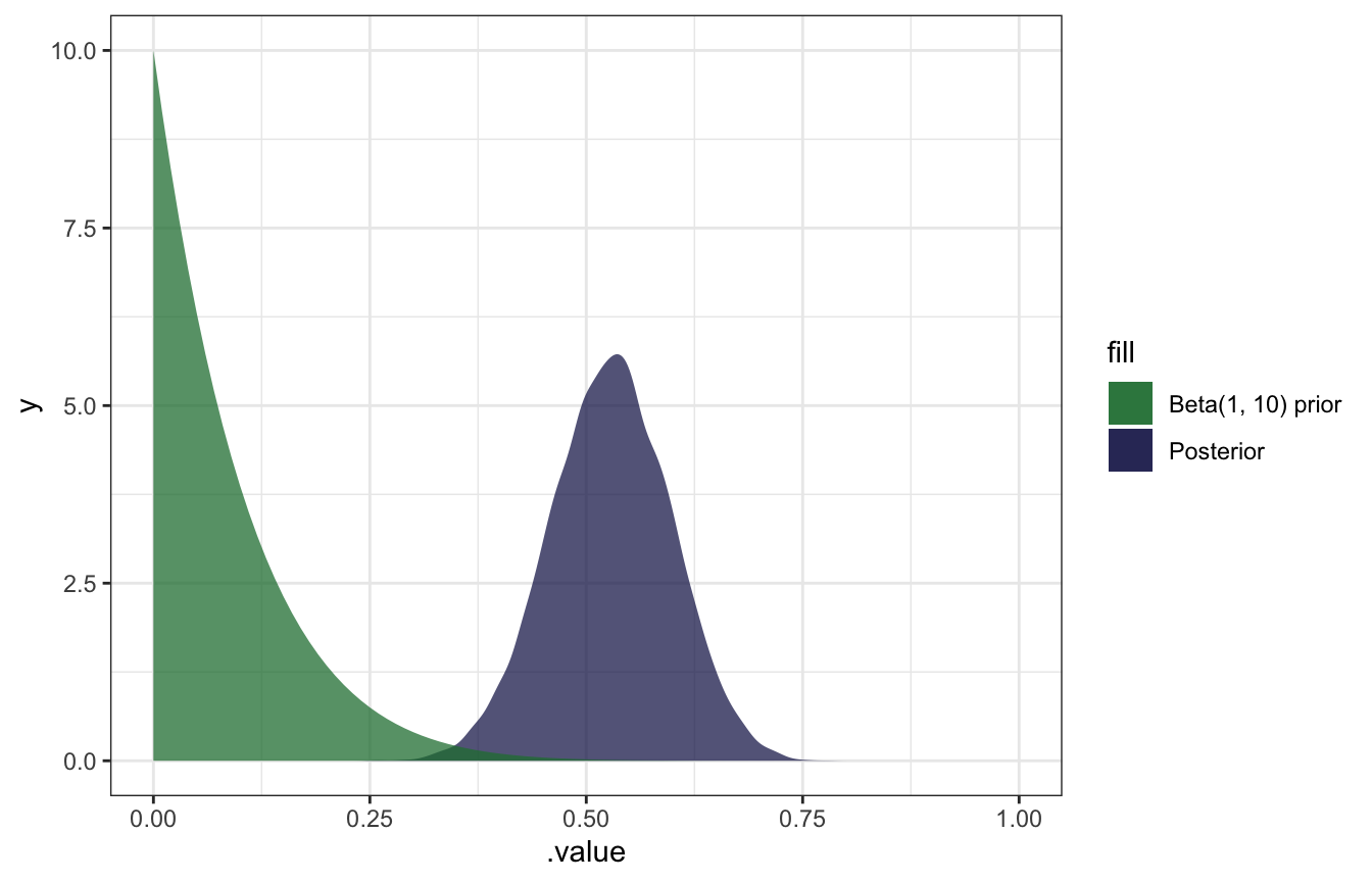
Milgram’s experiment

\[ \begin{aligned} Y \mid \pi &= \operatorname{Binomial}(40, \pi) \\ \pi &\sim \operatorname{Beta}(1, 10) \end{aligned} \]

model_milgram <- brm(
  bf(obey | trials(participants) ~ 0 + Intercept),
  data = list(obey = 26, participants = 40),
  family = binomial(link = "identity"),
  prior(beta(1, 10), class = b, lb = 0, ub = 1),
  iter = 5000, warmup = 1000, seed = BAYES_SEED,
  backend = "rstan", cores = 4
)
## Compiling Stan program...
## Start sampling

model_milgram %>% 
  gather_draws(b_Intercept) %>% 
  ggplot(aes(x = .value)) +
  geom_density(aes(fill = "Posterior"), color = NA, alpha = 0.75) +
  stat_function(geom = "area", fun = ~dbeta(., 1, 10), aes(fill = "Beta(1, 10) prior"), alpha = 0.75) +
  scale_fill_manual(values = clrs[5:6]) +
  xlim(c(0, 1))