2: Bayes’ Rule

Reading notes

Published

September 3, 2022

# Load packages
library(bayesrules)
library(tidyverse)
library(janitor)

# Import article data
data(fake_news)

perc <- scales::label_percent(accuracy = 1)
perc2 <- scales::label_percent(accuracy = 0.01)

How many are fake vs. real?

fake_news %>% 
  count(type) %>% 
  adorn_totals("row")
##   type   n
##   fake  60
##   real  90
##  Total 150

60/150 or 40% of news articles are fake .

How is the use of exclamation marks distributed across fake and real news articles?

fake_news %>% 
  tabyl(title_has_excl, type) %>% 
  adorn_totals("row")
##  title_has_excl fake real
##           FALSE   44   88
##            TRUE   16    2
##           Total   60   90

16/60 or 26.67% of news articles with !s are fake; only 2/90 or 2.22% of real articles with have !s.

Our prior is thus that 40% of news articles are fake. We have new data, that !s are more common in fake news articles. So what’s the posterior if we find an article with a !?

The chance that this article is fake jumps from 40% to roughly 90%. Though exclamation points are more common among fake articles, let’s not forget that only 40% of articles are fake.

Conditional probabilities

We have two variables:

Fake vs. real status
Use of exclamation points

These features can vary at random across different articles, so we have to represent that randomness with probabilities models

Prior probability model

We know from previous data that 40% are fake and 60% are real. If \(B\) means the article is fake, we can write that as

\[ P(B) = 0.40 \text{ and } P(B^c) = 0.60 \]

Conditional probability

The occurrence of !s depends on fakeness. Conditional probabilities of !s and fakeness, where \(A\) is the use of an exclamation mark:

\[ P(A \mid B) = 0.2667 \text{ and } P(A \mid B^c) = 0.0222 \]

By comparing conditional vs. unconditional probabilities, we learn how much \(B\) can inform our understanding of \(A\).

An event \(A\) might increase in probability given \(B\), like how the probability of joining an orchestra is greater if we know someonw practices daily:

\[ P(\text{join orchestra} \mid \text{practice daily}) > P(\text{join orchestra}) \]

Or the probability of getting the flu is lower if you know someone washes their hands a lot:

\[ P(\text{get flu} \mid \text{wash hands regularly}) < P(\text{get flu}) \]

Likelihood

Likelihood is kind of like the inverse of probability (not really! just that the order of A and B matters)

If we know \(B\), the conditional probability \(P(\cdot \mid B)\) lets us compare the probabilities of an unknown event \(A\) (or \(A^c\)) occurring with \(B\), or

\[ P(A \mid B) \text{ vs. } P(A^c \mid B) \]
If we know \(A\), the likelihood function \(L(\cdot \mid A) = P(A \mid \cdot)\) lets us compare the relative compatibility of data \(A\) with events \(B\) or \(B^c\)

\[ L(B \mid A) \text{ vs. } L(B^c \mid A) \]

What this looks like in practice, where \(A\) means having an exclamation mark and \(B\) means being fake:

# Prior probability
row_prior <- fake_news %>% 
  count(type) %>% 
  mutate(prop = n / sum(n)) %>% 
  select(-n) %>% 
  pivot_wider(names_from = type, values_from = prop)

# Likelihood
row_likelihood <- fake_news %>% 
  count(type, title_has_excl) %>% 
  pivot_wider(names_from = title_has_excl, values_from = n) %>% 
  mutate(likelihood = `TRUE` / (`TRUE` + `FALSE`)) %>% 
  select(-c(`FALSE`, `TRUE`)) %>%
  pivot_wider(names_from = type, values_from = likelihood)

bind_cols(Statistic = c("Prior probability", "Likelihood"),
          bind_rows(row_prior, row_likelihood)) %>% 
  mutate(Total = fake + real) %>% 
  rename(`Fake ($B$)` = fake, 
         `Real ($B^c$)` = real) %>% 
  knitr::kable(digits = 3)

Statistic	Fake (\(B\))	Real (\(B^c\))	Total
Prior probability	0.400	0.600	1.000
Likelihood	0.267	0.022	0.289

Normalizing constants

The last piece we need is the marginal probability of observing exclamation points across all articles, or \(P(A)\), which is the normalizing constant, or \(P(B)L(B \mid A) + P(B^c)L(B^c \mid A)\)

fake_news %>% 
  count(type, title_has_excl) %>% 
  mutate(prop = n / sum(n)) %>% 
  filter(title_has_excl == TRUE) %>% 
  summarize(normalizing_constant = sum(prop))
##   normalizing_constant
## 1                 0.12

Final analytical posterior

Thus, given this formula:

\[ \text{posterior} = \frac{\text{prior} \times \text{likelihood}}{\text{normalizing constant}} \]

…we have

\[ \text{posterior} = \frac{0.4 \times 0.2667}{0.12} = 0.889 \]

Simulation

We can simulate this too

sim_params <- tibble(type = c("real", "fake"),
                     prior = c(0.6, 0.4))

set.seed(1234)

sims <- sample(sim_params$type, size = 10000, prob = sim_params$prior, replace = TRUE) %>% 
  enframe(value = "type") %>% 
  mutate(data_model = case_when(type == "fake" ~ 0.2667,
                                type == "real" ~ 0.0222)) %>% 
  rowwise() %>% 
  mutate(usage = sample(c("no", "yes"), size = 1,
                        prob = c(1 - data_model, data_model))) %>% 
  ungroup()

sims %>% 
  tabyl(usage, type) %>% 
  adorn_totals(c("col", "row"))
##  usage fake real Total
##     no 2914 5872  8786
##    yes 1075  139  1214
##  Total 3989 6011 10000

ggplot(sims, aes(x = type, fill = usage)) +
  geom_bar(position = position_fill())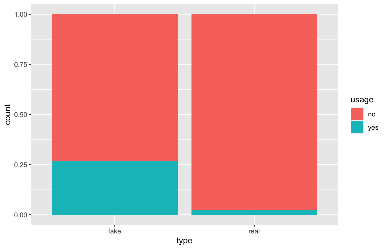


# Posterior
sims %>% 
  filter(usage == "yes") %>% 
  count(type) %>% 
  mutate(prop = n / sum(n))
## # A tibble: 2 × 3
##   type      n  prop
##   <chr> <int> <dbl>
## 1 fake   1075 0.886
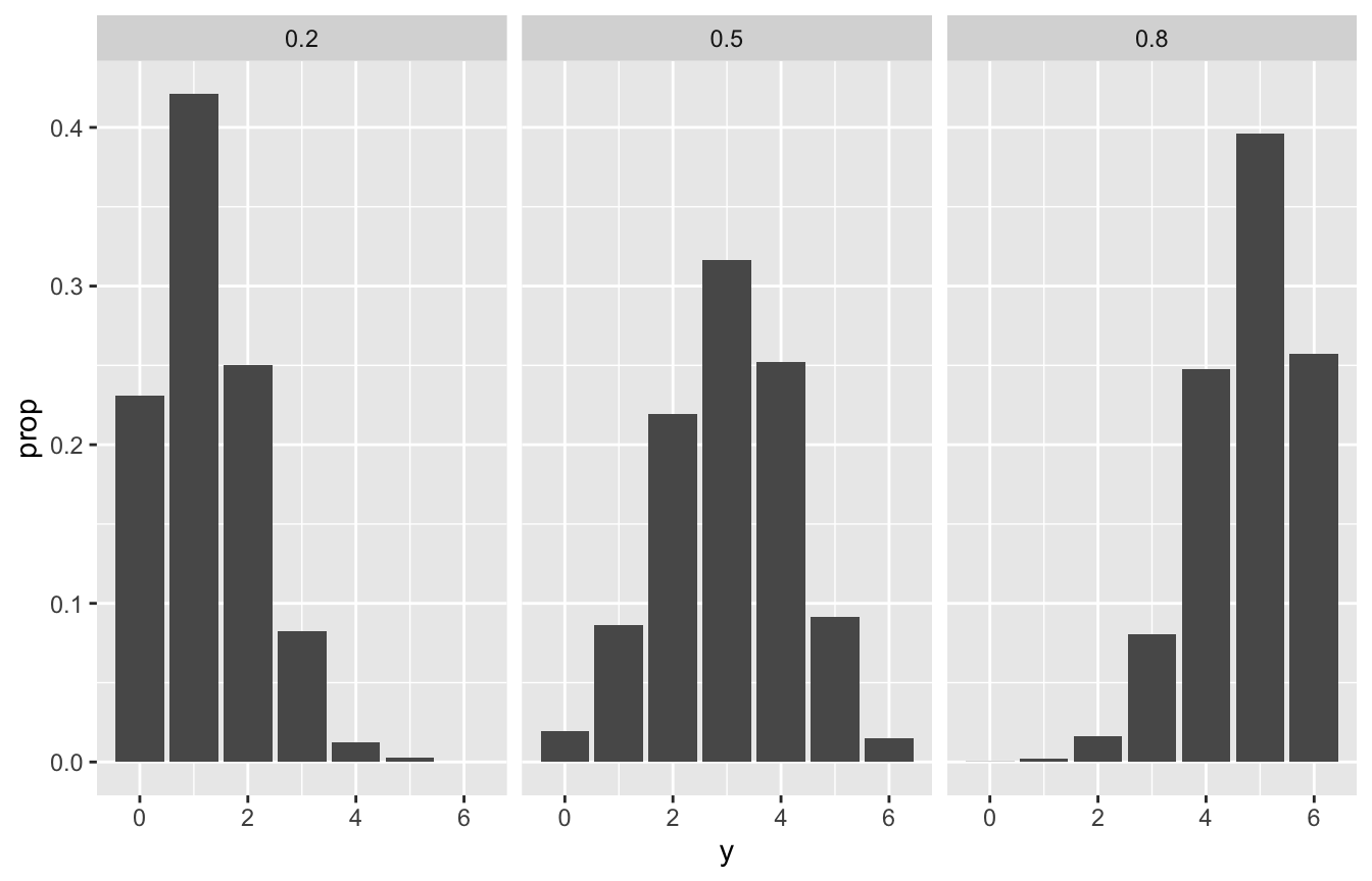
## 2 real    139 0.114

Chess simulation

chess <- c(0.2, 0.5, 0.8)
prior <- c(0.1, 0.25, 0.65)

set.seed(1234)
chess_sim <- tibble(pi = sample(chess, size = 10000, prob = prior, replace = TRUE)) %>% 
  mutate(y = rbinom(n(), size = 6, prob = pi))

chess_sim %>% 
  count(pi) %>% 
  mutate(prop = n / sum(n))
## # A tibble: 3 × 3
##      pi     n   prop
##   <dbl> <int>  <dbl>
## 1   0.2   986 0.0986
## 2   0.5  2523 0.252 
## 3   0.8  6491 0.649

chess_sim %>% 
  ggplot(aes(x = y)) +
  stat_count(aes(y = ..prop..)) +
  facet_wrap(vars(pi))
## Warning: The dot-dot notation (`..prop..`) was deprecated in ggplot2 3.4.0.
## ℹ Please use `after_stat(prop)` instead.