9: Simple normal regression

Reading notes

Published

October 4, 2022

library(bayesrules)
library(tidyverse)
library(brms)
library(cmdstanr)
library(rstanarm)
library(broom.mixed)
library(tidybayes)
library(ggdist)
library(patchwork)
library(ggtext)

# Plot stuff
clrs <- MetBrewer::met.brewer("Lakota", 6)
theme_set(theme_bw())

# Seed stuff
set.seed(1234)
BAYES_SEED <- 1234

data(bikes, package = "bayesrules")

bikes <- bikes |> 
  mutate(temp_feel_centered = scale(temp_feel, scale = FALSE),
         temp_feel_c = as.numeric(temp_feel_centered))

temp_details <- attributes(bikes$temp_feel_centered) %>%
  set_names(janitor::make_clean_names(names(.)))

9.2: Tuning prior models for regression parameters

We want to estimate the effect of temperature on bike share ridership. We need to estimate three parameters:

\(\beta_0\), or the intercept. From prior research, we know:

On an average temperature day, say 65 or 70 degrees for D.C., there are typically around 5000 riders, though this average could be somewhere between 3000 and 7000.

\(\beta_1\), or the slope. From prior research, we know:

For every one degree increase in temperature, ridership typically increases by 100 rides, though this average increase could be as low as 20 or as high as 180.

\(\sigma\), or the variation in ridership. From prior research, we know:

At any given temperature, daily ridership will tend to vary with a moderate standard deviation of 1250 rides.

The intercept there is centered at 5000 riders.

That gives us these priors:

p1 <- ggplot() +
  geom_function(fun = ~dnorm(., 5000, 1000), size = 1, color = clrs[1]) +
  xlim(c(1000, 9000)) +
  labs(x = "**β<sub>0c</sub>**<br>Average daily ridership, centered") +
  theme(axis.title.x = element_markdown())
## Warning: Using `size` aesthetic for lines was deprecated in ggplot2 3.4.0.
## ℹ Please use `linewidth` instead.

p2 <- ggplot() +
  geom_function(fun = ~dnorm(., 100, 40), size = 1, color = clrs[3]) +
  xlim(c(-50, 250)) +
  labs(x = "**β<sub>1</sub>**<br>Effect of temperature on ridership") +
  theme(axis.title.x = element_markdown())

p3 <- ggplot() +
  geom_function(fun = ~dexp(., 1 / 1250), size = 1, color = clrs[4]) +
  xlim(c(0, 7000)) +
  labs(x = "**σ**<br>Variation in daily ridership") +
  theme(axis.title.x = element_markdown())

p1 | p2 | p3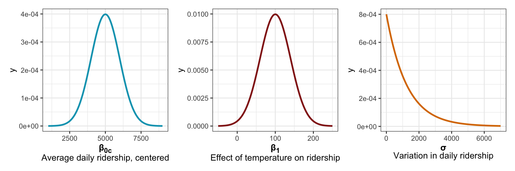

More formally, we can write out the whole model like this:

\[ \begin{aligned} Y_i &\sim \mathcal{N}(\mu_i, \sigma) \text{, or} & \text{[McElreath's syntax]} \\ Y_i \mid \beta_0, \beta_1, \sigma &\stackrel{\text{ind}}{\sim} \mathcal{N}(\mu_i, \sigma^2) & \text{[Bayes Rules!'s syntax]} \\ \mu_i &= \beta_{0c} + \beta_1 X_i \\ \\ \beta_{0c} &\sim \mathcal{N}(5000, 1000) \\ \beta_{1} &\sim \mathcal{N}(100, 40) \\ \sigma &\sim \operatorname{Exponential}(1 / 1250) \end{aligned} \]

We can simulate from all these priors to see how reasonable they are, McElreath-style. In Bayes Rules! they show a picture of this but not the code to make it. I’ll use brms bc it’s easy.

priors <- c(prior(normal(5000, 1000), class = Intercept),
            prior(normal(100, 40), class = b, coef = "temp_feel_c"),
            prior(exponential(0.0008), class = sigma))

bike_prior_only <- brm(
  bf(rides ~ temp_feel_c),
  data = bikes,
  family = gaussian(),
  prior = priors,
  sample_prior = "only",
  backend = "cmdstanr", cores = 4, seed = BAYES_SEED, refresh = 0
)
## Start sampling

These lines all look reasonable, yay.

draws_prior <- tibble(temp_feel_c = seq(45 - temp_details$scaled_center, 
                                        90 - temp_details$scaled_center, 
                                        1)) |> 
  add_epred_draws(bike_prior_only, ndraws = 200) |> 
  mutate(unscaled = temp_feel_c + temp_details$scaled_center)

draws_prior |> 
  ggplot(aes(x = unscaled, y = .epred)) +
  geom_line(aes(group = .draw), alpha = 0.2) +
  labs(x = "Temperature", y = "Number of rides")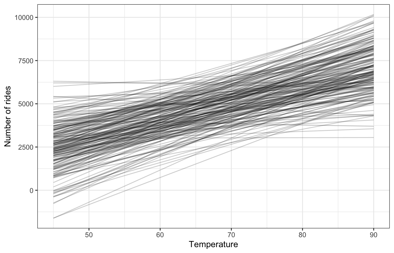

9.3: Posterior simulation

Run the model

bike_rstanarm <- stan_glm(
  rides ~ temp_feel_c,
  data = bikes,
  family = gaussian(),
  prior_intercept = normal(5000, 1000),
  prior = normal(100, 40),
  prior_aux = exponential(0.0008),
  chains = 4, iter = 5000*2, seed = 84735, refresh = 0
)

priors <- c(prior(normal(5000, 1000), class = Intercept),
            prior(normal(100, 40), class = b, coef = "temp_feel_c"),
            prior(exponential(0.0008), class = sigma))

bike_brms <- brm(
  bf(rides ~ temp_feel_c),
  data = bikes,
  family = gaussian(),
  prior = priors,
  chains = 4, iter = 5000*2, seed = BAYES_SEED, 
  backend = "cmdstanr", refresh = 0,
  file = "09-manual_cache/bike-brms"
)
## Start sampling

09-stan/bike-simple.stan

data {
  int<lower = 0> n;
  vector[n] Y;
  vector[n] X;
}

/*
// We could also center things here and then use it in mu below:
// mu = beta0 + beta1 * X_centered;
// See https://mc-stan.org/docs/stan-users-guide/standardizing-predictors-and-outputs.html
transformed data {
  vector[n] X_centered;
  
  X_centered = X - mean(X);
}
*/

parameters {
  real beta0;
  real beta1;
  real<lower = 0> sigma;
}

transformed parameters {
  vector[n] mu;
  mu = beta0 + beta1 * X;
}

model {
  Y ~ normal(mu, sigma);
  
  beta0 ~ normal(5000, 1000);
  beta1 ~ normal(100, 40);
  sigma ~ exponential(0.0008);
}

generated quantities {
  vector[n] Y_rep;
  
  for (i in 1:n) {
    Y_rep[i] = normal_rng(mu[i], sigma);
  }
}

bike_stan <- cmdstan_model("09-stan/bike-simple.stan")

bike_stan_samples <- bike_stan$sample(
  data = list(n = nrow(bikes), Y = bikes$rides, X = bikes$temp_feel_c),
  parallel_chains = 4, iter_warmup = 5000, iter_sampling = 5000, 
  refresh = 0, seed = BAYES_SEED,
  output_dir = "09-stan"
)
## Running MCMC with 4 parallel chains...
## 
## Chain 1 finished in 2.0 seconds.
## Chain 3 finished in 2.0 seconds.
## Chain 4 finished in 2.0 seconds.
## Chain 2 finished in 2.0 seconds.
## 
## All 4 chains finished successfully.
## Mean chain execution time: 2.0 seconds.
## Total execution time: 2.1 seconds.

Diagnostics

Effective sample size and R-hat

neff_ratio(bike_rstanarm)
## (Intercept) temp_feel_c       sigma 
##     0.96345     0.96075     0.96825
rhat(bike_rstanarm)
## (Intercept) temp_feel_c       sigma 
##   0.9998765   0.9999727   1.0000086

Trace plots

bike_rstanarm |> 
  gather_draws(`(Intercept)`, temp_feel_c, sigma) |> 
  ungroup() |> 
  mutate(.variable = fct_relevel(factor(.variable), c("(Intercept)", "temp_feel_c", "sigma"))) |> 
  ggplot(aes(x = .iteration, y = .value, color = as.factor(.chain))) +
  geom_line(size = 0.05) +
  labs(color = "Chain") +
  facet_wrap(vars(.variable), scales = "free_y") +
  theme(legend.position = "bottom")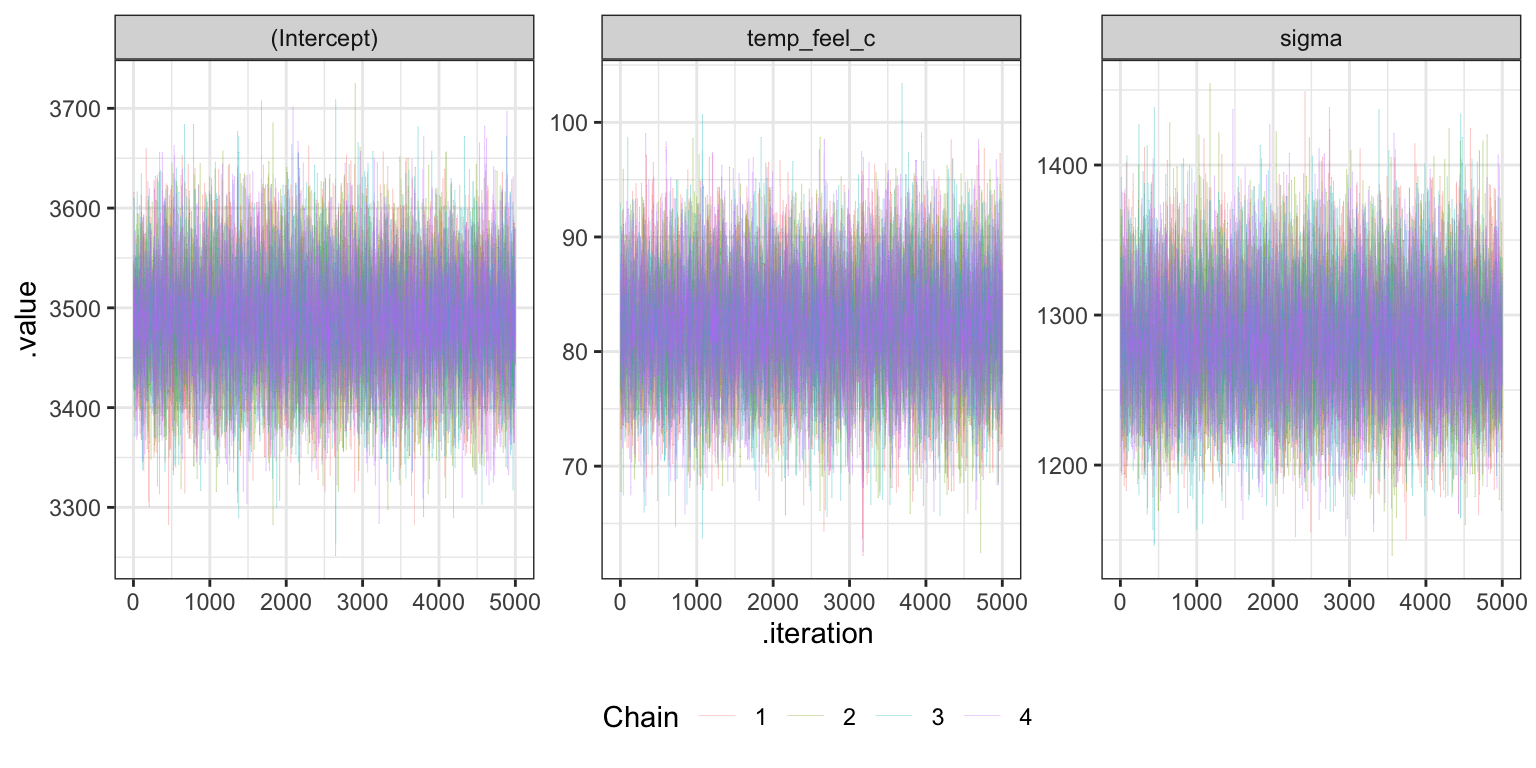

Trank plots

bike_rstanarm |> 
  gather_draws(`(Intercept)`, temp_feel_c, sigma) |> 
  ungroup() |> 
  mutate(.variable = fct_relevel(factor(.variable), c("(Intercept)", "temp_feel_c", "sigma"))) |> 
  group_by(.variable) |> 
  mutate(draw_rank = rank(.value)) |> 
  ggplot(aes(x = draw_rank)) +
  stat_bin(aes(color = factor(.chain)), geom = "step", binwidth = 1000,
           position = position_identity(), boundary = 0) +
  labs(color = "Chain") +
  facet_wrap(vars(.variable)) +
  theme(legend.position = "bottom",
        axis.text.y = element_blank(), axis.title.y = element_blank(), axis.ticks.y = element_blank())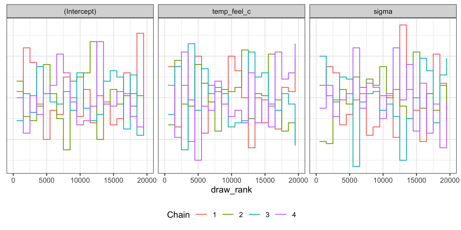

Density plots

bike_rstanarm |> 
  gather_draws(`(Intercept)`, temp_feel_c, sigma) |> 
  ungroup() |> 
  mutate(.variable = fct_relevel(factor(.variable), c("(Intercept)", "temp_feel_c", "sigma"))) |> 
  ggplot(aes(x = .value, color = factor(.chain))) +
  geom_density() +
  labs(color = "Chain") +
  facet_wrap(vars(.variable), scales = "free") +
  theme(legend.position = "bottom")

Effective sample size and R-hat

neff_ratio(bike_brms)
##   b_Intercept b_temp_feel_c         sigma        lprior          lp__ 
##     1.0579051     1.0534749     1.1040274     1.0473025     0.4827253
rhat(bike_brms)
##   b_Intercept b_temp_feel_c         sigma        lprior          lp__ 
##      1.000021      1.000172      1.000024      1.000135      1.000185

Trace plots

bike_brms |> 
  gather_draws(b_Intercept, b_temp_feel_c, sigma) |> 
  ggplot(aes(x = .iteration, y = .value, color = as.factor(.chain))) +
  geom_line(size = 0.05) +
  labs(color = "Chain") +
  facet_wrap(vars(.variable), scales = "free_y") +
  theme(legend.position = "bottom")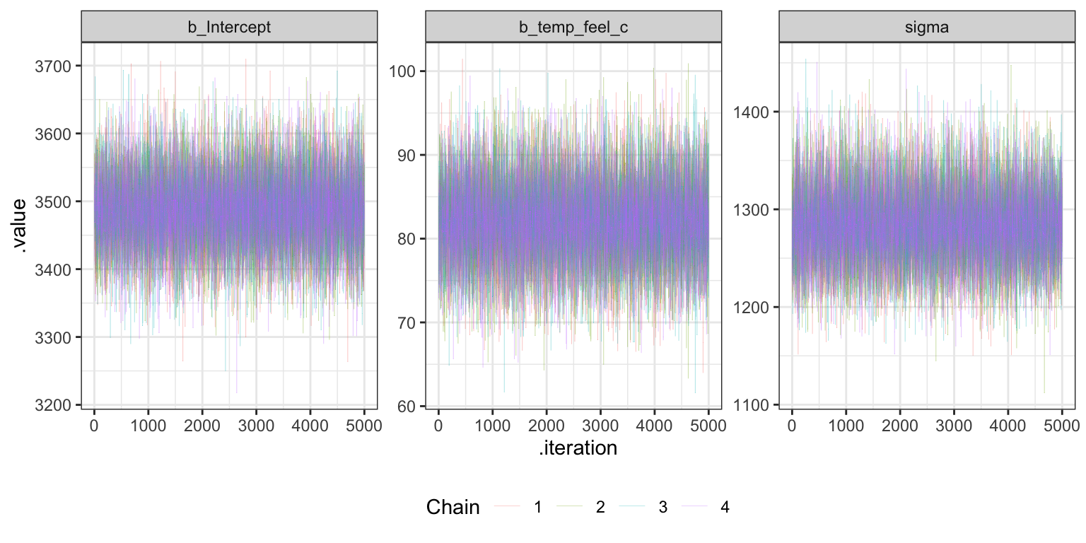

Trank plots

bike_brms |> 
  gather_draws(b_Intercept, b_temp_feel_c, sigma) |> 
  group_by(.variable) |> 
  mutate(draw_rank = rank(.value)) |> 
  ggplot(aes(x = draw_rank)) +
  stat_bin(aes(color = factor(.chain)), geom = "step", binwidth = 1000,
           position = position_identity(), boundary = 0) +
  labs(color = "Chain") +
  facet_wrap(vars(.variable)) +
  theme(legend.position = "bottom",
        axis.text.y = element_blank(), axis.title.y = element_blank(), axis.ticks.y = element_blank())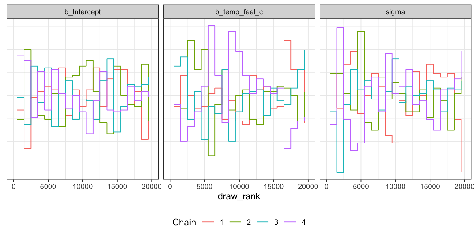

Density plots

bike_brms |> 
  gather_draws(b_Intercept, b_temp_feel_c, sigma) |> 
  ggplot(aes(x = .value, color = factor(.chain))) +
  geom_density() +
  labs(color = "Chain") +
  facet_wrap(vars(.variable), scales = "free") +
  theme(legend.position = "bottom")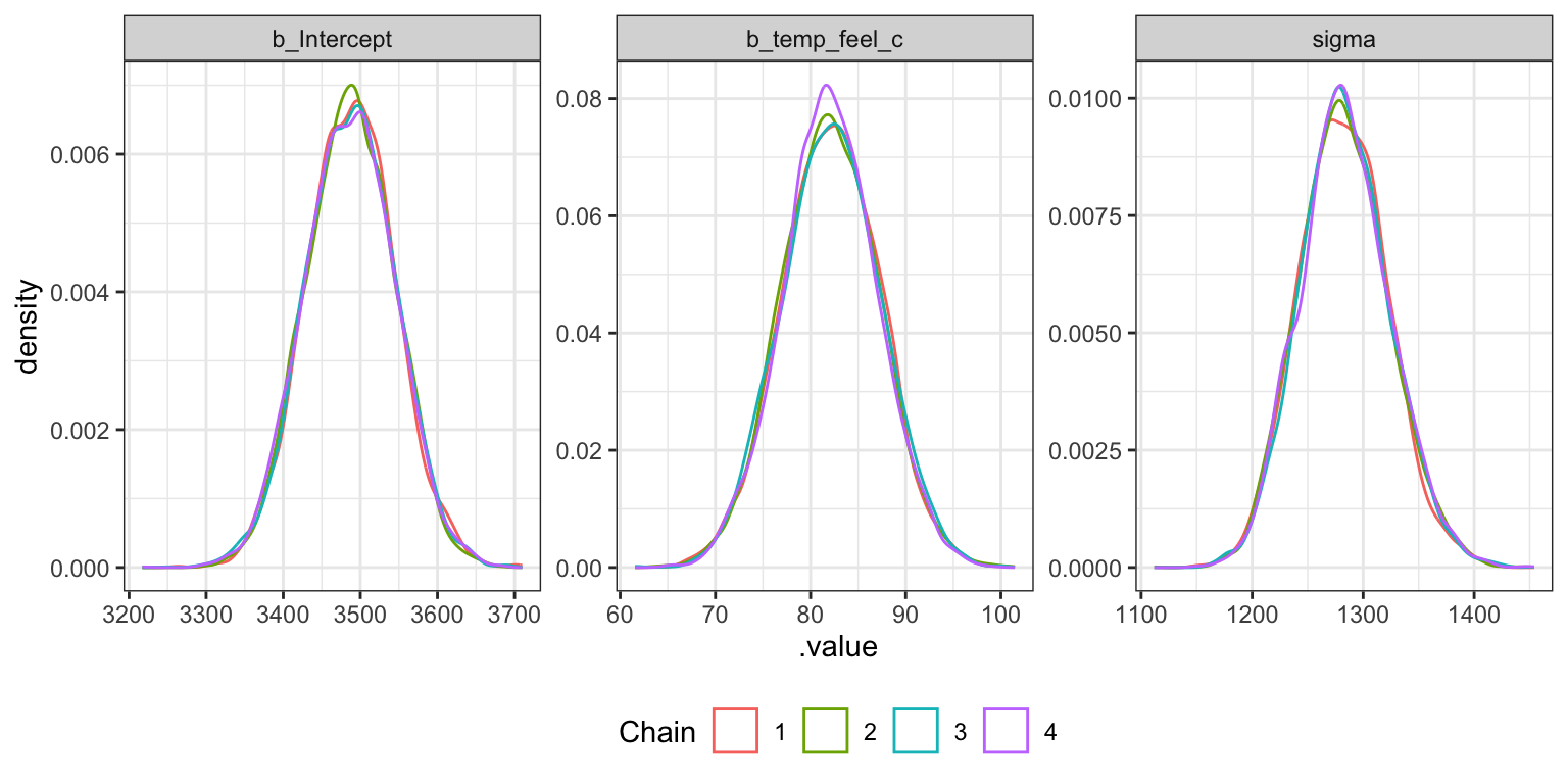

Effective sample size and R-hat

neff_ratio(bike_stan_samples, pars = c("beta0", "beta1", "sigma"))
##    beta0    beta1    sigma 
## 1.077305 1.012467 1.085847
rhat(bike_stan_samples, pars = c("beta0", "beta1", "sigma"))
##     beta0     beta1     sigma 
## 1.0001360 1.0000768 0.9999753

Trace plots

bike_stan_samples |> 
  gather_draws(beta0, beta1, sigma) |> 
  ggplot(aes(x = .iteration, y = .value, color = as.factor(.chain))) +
  geom_line(size = 0.05) +
  labs(color = "Chain") +
  facet_wrap(vars(.variable), scales = "free_y") +
  theme(legend.position = "bottom")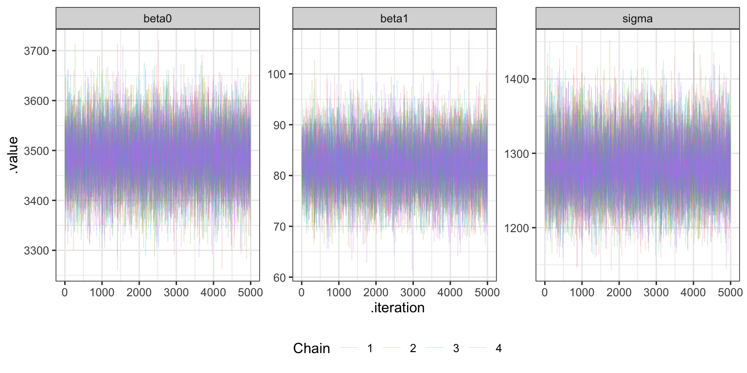

Trank plots

bike_stan_samples |> 
  gather_draws(beta0, beta1, sigma) |> 
  group_by(.variable) |> 
  mutate(draw_rank = rank(.value)) |> 
  ggplot(aes(x = draw_rank)) +
  stat_bin(aes(color = factor(.chain)), geom = "step", binwidth = 1000,
           position = position_identity(), boundary = 0) +
  labs(color = "Chain") +
  facet_wrap(vars(.variable)) +
  theme(legend.position = "bottom",
        axis.text.y = element_blank(), axis.title.y = element_blank(), axis.ticks.y = element_blank())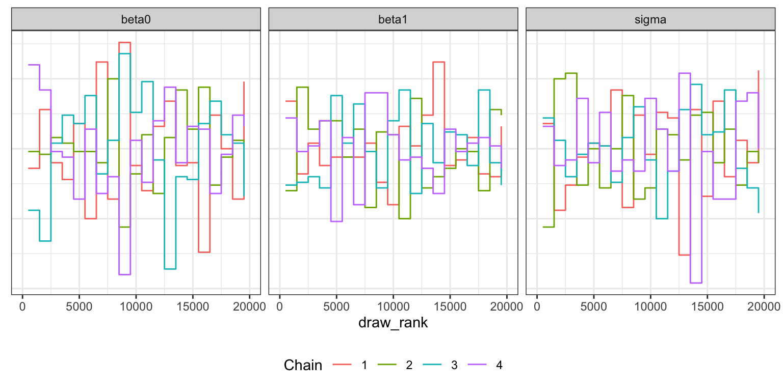

Density plots

bike_stan_samples |> 
  gather_draws(beta0, beta1, sigma) |> 
  ggplot(aes(x = .value, color = factor(.chain))) +
  geom_density() +
  labs(color = "Chain") +
  facet_wrap(vars(.variable), scales = "free") +
  theme(legend.position = "bottom")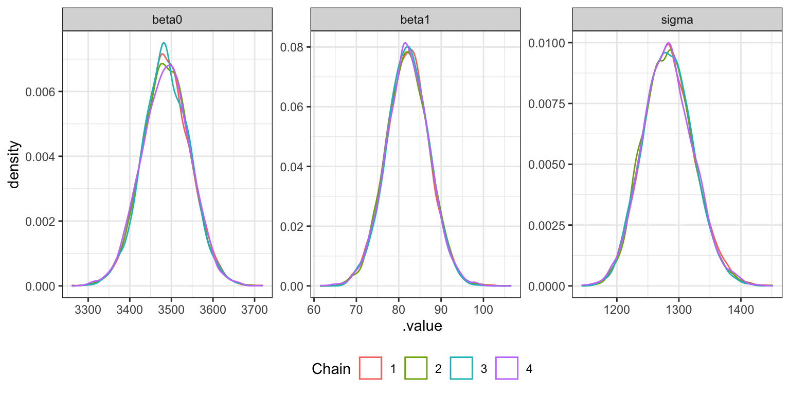

9.4: Interpreting the posterior

Parameter summaries

tidy(bike_rstanarm, effects = c("fixed", "aux"), 
     conf.int = TRUE, conf.level = 0.8)
## # A tibble: 4 × 5
##   term        estimate std.error conf.low conf.high
##   <chr>          <dbl>     <dbl>    <dbl>     <dbl>
## 1 (Intercept)   3487.      58.0    3413.     3561. 
## 2 temp_feel_c     82.2      5.08     75.7      88.7
## 3 sigma         1282.      40.9    1231.     1336. 
## 4 mean_PPD      3487.      82.0    3382.     3593.

bike_rstanarm |> 
  gather_draws(`(Intercept)`, temp_feel_c, sigma) |> 
  ungroup() |> 
  mutate(.variable = fct_relevel(factor(.variable), c("(Intercept)", "temp_feel_c", "sigma"))) |> 
  ggplot(aes(x = .value, fill = .variable)) +
  stat_halfeye(normalize = "xy") +
  scale_fill_manual(values = c(clrs[1], clrs[3], clrs[4]), guide = "none") +
  facet_wrap(vars(.variable), scales = "free_x") +
  labs(x = "Parameter posterior") +
  theme(legend.position = "bottom")
## Warning: Unknown or uninitialised column: `linewidth`.
## Warning: Using the `size` aesthietic with geom_segment was deprecated in ggplot2 3.4.0.
## ℹ Please use the `linewidth` aesthetic instead.
## Warning: Unknown or uninitialised column: `linewidth`.
## Unknown or uninitialised column: `linewidth`.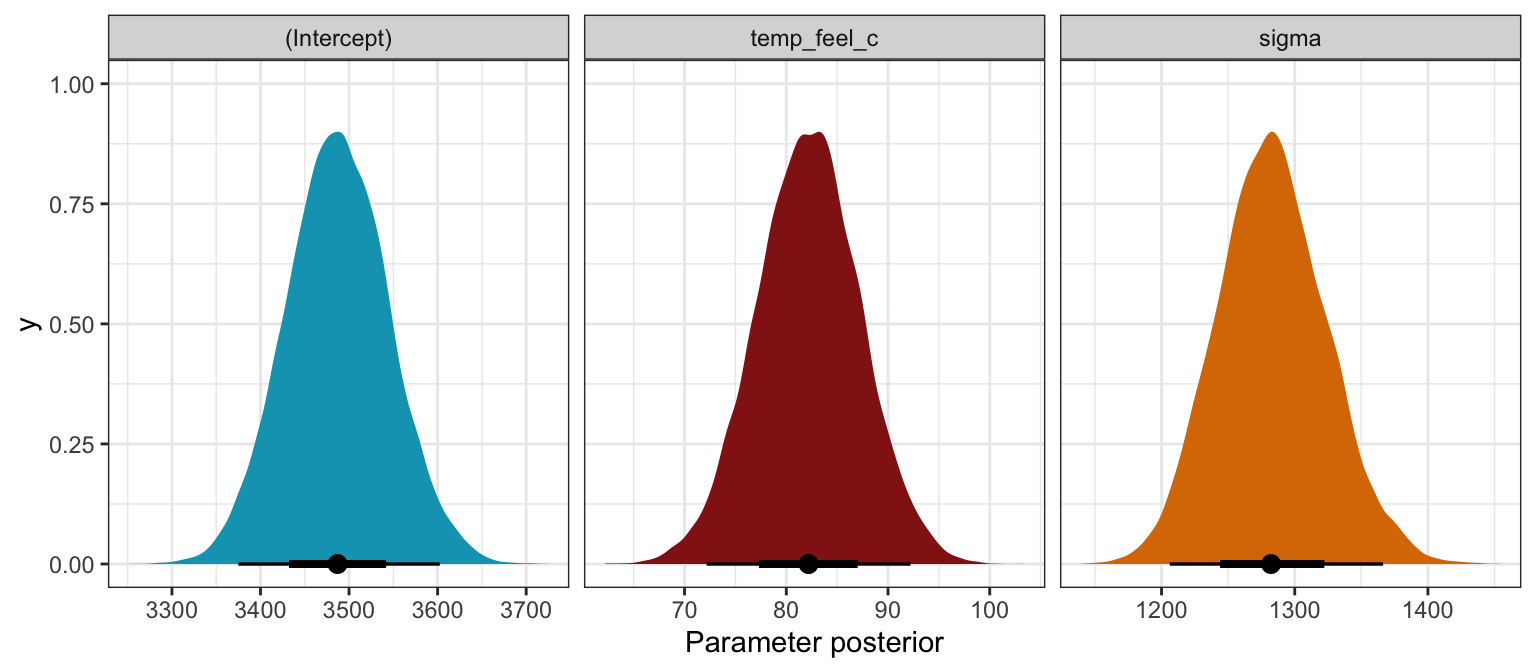

tidy(bike_brms, conf.int = TRUE, conf.level = 0.8) |> 
  select(-c(effect, component, group))
## # A tibble: 3 × 5
##   term            estimate std.error conf.low conf.high
##   <chr>              <dbl>     <dbl>    <dbl>     <dbl>
## 1 (Intercept)       3487.      57.5    3414.     3561. 
## 2 temp_feel_c         82.1      5.08     75.6      88.6
## 3 sd__Observation   1283.      40.3    1232.     1336.

bike_brms |> 
  gather_draws(b_Intercept, b_temp_feel_c, sigma) |> 
  ggplot(aes(x = .value, fill = .variable)) +
  stat_halfeye(normalize = "xy") +
  scale_fill_manual(values = c(clrs[1], clrs[3], clrs[4]), guide = "none") +
  facet_wrap(vars(.variable), scales = "free_x") +
  labs(x = "Parameter posterior") +
  theme(legend.position = "bottom")
## Warning: Unknown or uninitialised column: `linewidth`.
## Unknown or uninitialised column: `linewidth`.
## Unknown or uninitialised column: `linewidth`.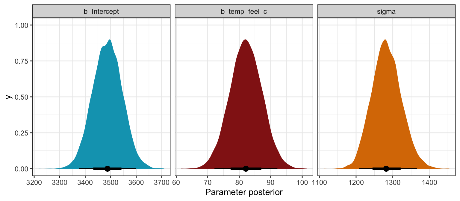

bike_stan_samples$print(variables = c("beta0", "beta1", "sigma"), 
                        "mean", "median", "sd", ~quantile(.x, probs = c(0.1, 0.9)))
##  variable    mean  median    sd     10%     90%
##     beta0 3487.16 3486.85 57.13 3414.32 3560.02
##     beta1   82.12   82.10  5.06   75.68   88.58
##     sigma 1282.72 1281.84 40.44 1231.39 1335.31

bike_stan_samples |> 
  gather_draws(beta0, beta1, sigma) |> 
  ggplot(aes(x = .value, fill = .variable)) +
  stat_halfeye(normalize = "xy") +
  scale_fill_manual(values = c(clrs[1], clrs[3], clrs[4]), guide = "none") +
  facet_wrap(vars(.variable), scales = "free_x") +
  labs(x = "Parameter posterior") +
  theme(legend.position = "bottom")
## Warning: Unknown or uninitialised column: `linewidth`.
## Unknown or uninitialised column: `linewidth`.
## Unknown or uninitialised column: `linewidth`.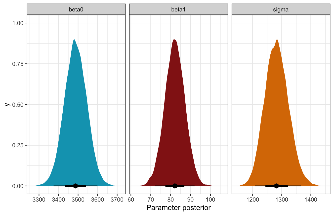

Fitted draws

bikes |> 
  add_linpred_draws(bike_rstanarm, ndraws = 100) |> 
  ggplot(aes(x = temp_feel, y = rides)) +
  geom_point(data = bikes, size = 0.5) +
  geom_line(aes(y = .linpred, group = .draw), alpha = 0.2, size = 0.5, color = clrs[6]) +
  labs(x = "Temperature", y = "Rides")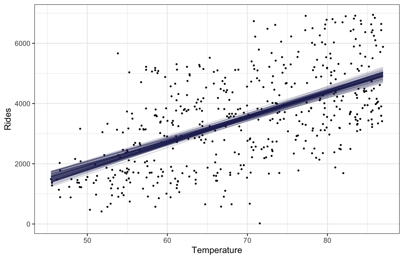

bikes |> 
  add_linpred_draws(bike_brms, ndraws = 100) |> 
  ggplot(aes(x = temp_feel, y = rides)) +
  geom_point(data = bikes, size = 0.5) +
  geom_line(aes(y = .linpred, group = .draw), alpha = 0.2, size = 0.5, color = clrs[6]) +
  labs(x = "Temperature", y = "Rides")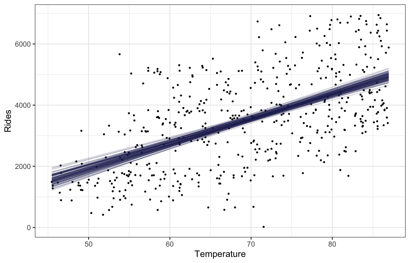

bike_stan_samples |> 
  spread_draws(mu[i]) |> 
  mean_qi() |> 
  bind_cols(bikes) |> 
  ggplot(aes(x = temp_feel, y = rides)) +
  geom_point(size = 0.5) +
  geom_line(aes(y = mu), color = clrs[6], size = 1) +
  geom_ribbon(aes(ymin = .lower, ymax = .upper), fill = clrs[6], alpha = 0.2) +
  labs(x = "Temperature", y = "Rides")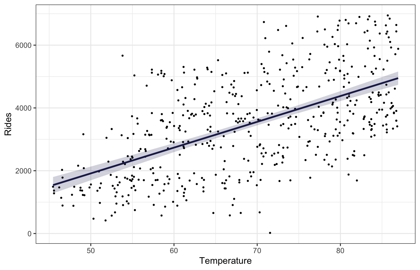

There’s no easy way to replicate add_linpred_draws(..., ndraws = BLAH) with raw Stan like this without running the model again and generating a bunch of simulated mus based on some variable like n_sim that we build into the Stan model, but we can use the original 500 rows of data and use geom_lineribbon() instead of a spaghetti plot.

Is β₁ > 0?

Easily.

bike_rstanarm |> 
  spread_draws(temp_feel_c) |> 
  count(temp_feel_c > 0) |> 
  mutate(prob = n / sum(n))
## # A tibble: 1 × 3
##   `temp_feel_c > 0`     n  prob
##   <lgl>             <int> <dbl>
## 1 TRUE              20000     1

bike_brms |> 
  spread_draws(b_temp_feel_c) |> 
  count(b_temp_feel_c > 0) |> 
  mutate(prob = n / sum(n))
## # A tibble: 1 × 3
##   `b_temp_feel_c > 0`     n  prob
##   <lgl>               <int> <dbl>
## 1 TRUE                20000     1

bike_stan_samples |> 
  spread_draws(beta1) |> 
  count(beta1 > 0) |> 
  mutate(prob = n / sum(n))
## # A tibble: 1 × 3
##   `beta1 > 0`     n  prob
##   <lgl>       <int> <dbl>
## 1 TRUE        20000     1

9.5: Posterior prediction

We could plug in some temperature, like 75, and get a predicted count of riders (values from the rstanarm model):

values_rstanarm <- bike_rstanarm |> 
  tidy() |> 
  split(~term)

b0 <- values_rstanarm$`(Intercept)`$estimate
b1 <- values_rstanarm$temp_feel_c$estimate
temp_mean <- temp_details$scaled_center

b0 + (b1 * (75 - temp_mean))
## [1] 3968.317

But this ignores two types of uncertainty:

Sampling variability in the data, or in \(Y\)
Posterior variability in parameters, or in \(\beta_0\), \(\beta_1\), and \(\sigma\)

p1 <- bike_rstanarm |> 
  linpred_draws(newdata = tibble(temp_feel_c = (75 - temp_mean))) |> 
  ggplot(aes(x = .linpred)) +
  stat_halfeye(fill = clrs[6]) +
  labs(title = "Predicted riders at 75˚",
       subtitle = "µ only; posterior_linpred()",
       x = "Predicted riders", y = NULL)

p2 <- bike_rstanarm |> 
  predicted_draws(newdata = tibble(temp_feel_c = (75 - temp_mean))) |> 
  ggplot(aes(x = .prediction)) +
  stat_halfeye(fill = clrs[5]) +
  labs(title = "Predicted riders at 75˚",
       subtitle = "rnorm(µ, σ); posterior_predict()",
       x = "Predicted riders", y = NULL)

p1 | p2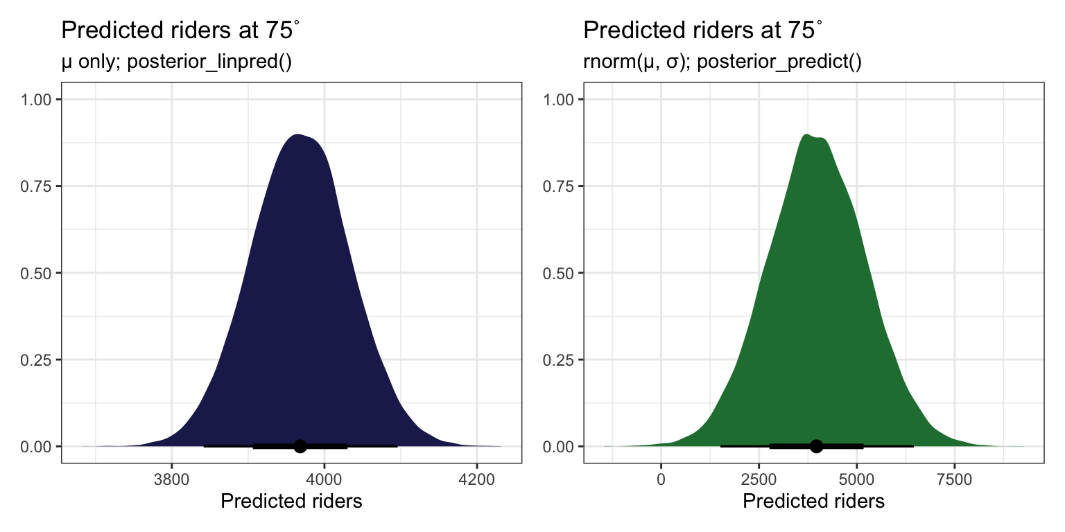

p1 <- bike_brms |> 
  linpred_draws(newdata = tibble(temp_feel_c = (75 - temp_mean))) |> 
  ggplot(aes(x = .linpred)) +
  stat_halfeye(fill = clrs[6]) +
  labs(title = "Predicted riders at 75˚",
       subtitle = "µ only; posterior_linpred()",
       x = "Predicted riders", y = NULL)

p2 <- bike_brms |> 
  predicted_draws(newdata = tibble(temp_feel_c = (75 - temp_mean))) |> 
  ggplot(aes(x = .prediction)) +
  stat_halfeye(fill = clrs[5]) +
  labs(title = "Predicted riders at 75˚",
       subtitle = "rnorm(µ, σ); posterior_predict()",
       x = "Predicted riders", y = NULL)

p1 | p2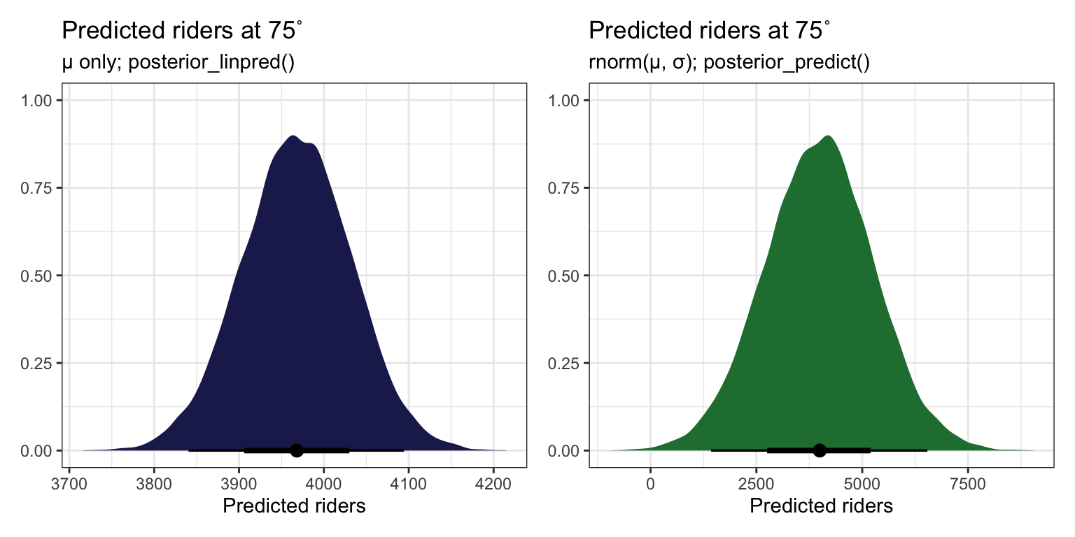

AHH SO THIS IS HOW YOU DO newdata = WHATEVER WITH RAW STAN. Build mu (posterior_linpred()) on your own with the coefficients from each draw, then use that mu in rnorm() (posterior_predict()). You can then get the expectation of the posterior (posterior_epred()) by taking the average of that.

predict_75 <- bike_stan_samples |> 
  spread_draws(beta0, beta1, sigma) |> 
  mutate(mu = beta0 + (beta1 * (75 - temp_mean)),  # like posterior_linpred()
         y_new = rnorm(n(), mean = mu, sd = sigma))  # like posterior_predict()

p1 <- predict_75 |> 
  ggplot(aes(x = mu)) +
  stat_halfeye(fill = clrs[6]) +
  labs(title = "Predicted riders at 75˚",
       subtitle = "µ only; like posterior_linpred()",
       x = "Predicted riders", y = NULL)

p2 <- predict_75 |> 
  ggplot(aes(x = y_new)) +
  stat_halfeye(fill = clrs[5]) +
  labs(title = "Predicted riders at 75˚",
       subtitle = "rnorm(µ, σ); like posterior_predict()",
       x = "Predicted riders", y = NULL)

p1 | p2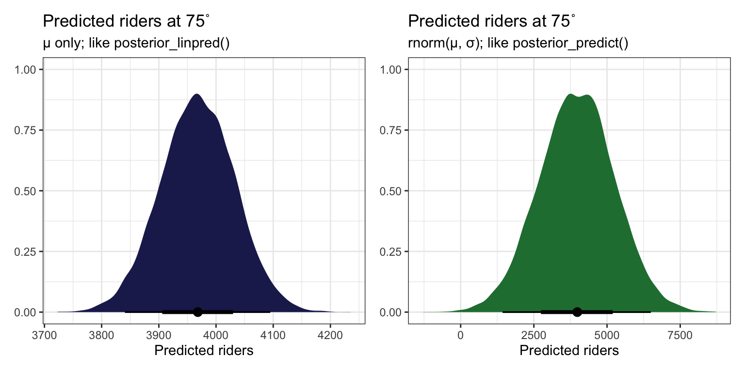


predict_75 |> 
  summarize(epred = mean(y_new))
## # A tibble: 1 × 1
##   epred
##   <dbl>
## 1 3974.

9.6: Sequential regression modeling

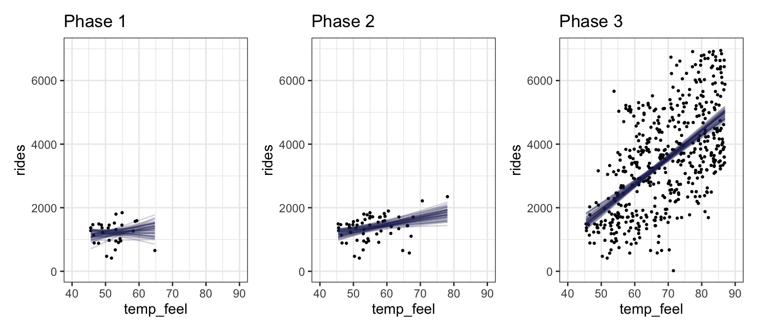
Bayesianism is all about updating. What does this relationship between temperature and ridership as data is slowly collected, like after 30 days, 60 days, and 500 days? How does the posterior evolve and settle?

I’ll do this just with brms:

priors <- c(prior(normal(5000, 1000), class = Intercept),
            prior(normal(100, 40), class = b, coef = "temp_feel_c"),
            prior(exponential(0.0008), class = sigma))

bike_phases <- tribble(
  ~phase, ~data,
  1,      slice(bikes, 1:30),
  2,      slice(bikes, 1:60),
  3,      bikes
) |> 
  mutate(model = map(data, ~{
    brm(
      bf(rides ~ temp_feel_c),
      data = .,
      family = gaussian(),
      prior = priors,
      chains = 4, iter = 5000*2, seed = BAYES_SEED, 
      backend = "cmdstanr", refresh = 0
    )})
  )
## Start sampling
## Start sampling
## Start sampling

bike_phase_draws <- bike_phases |> 
  mutate(draws = map(model, ~spread_draws(., b_temp_feel_c)))

phases_coefs <- bike_phase_draws |> 
  mutate(coef_plot = map2(draws, phase, ~{
    ggplot(.x, aes(x = b_temp_feel_c)) +
      stat_halfeye(fill = clrs[3]) +
      coord_cartesian(xlim = c(-10, 100)) +
      labs(title = paste("Phase", .y))
  }))

wrap_plots(phases_coefs$coef_plot)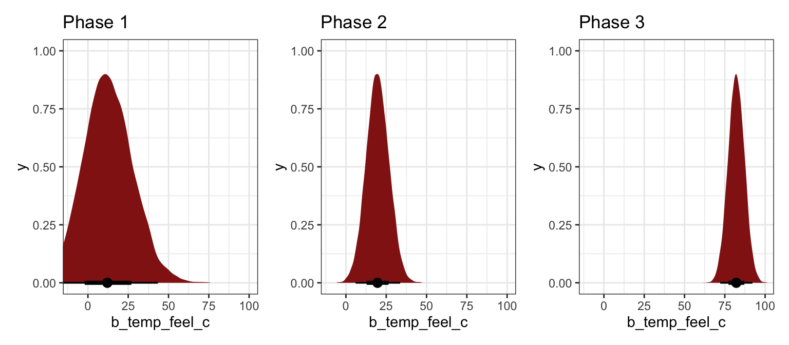

bike_phase_preds <- bike_phases |> 
  mutate(preds = map2(data, model, ~{
    .x |> 
      add_linpred_draws(.y, ndraws = 50) |> 
      ungroup()
  }))

phases_preds <- bike_phase_preds |> 
  mutate(pred_plot = pmap(list(data, preds, phase), ~{
    ggplot(..2, aes(x = temp_feel, y = rides)) +
      geom_point(data = ..1, size = 0.5) +
      geom_line(aes(y = .linpred, group = .draw), 
                alpha = 0.2, size = 0.5, color = clrs[6]) +
      labs(title = paste("Phase", ..3)) +
      coord_cartesian(xlim = c(40, 90), ylim = c(0, 7000))
  }))

wrap_plots(phases_preds$pred_plot)

9.2: Tuning prior models for regression parameters

9.3: Posterior simulation

Run the model

Diagnostics

Effective sample size and R-hat

Trace plots

Trank plots

Density plots

Effective sample size and R-hat

Trace plots

Trank plots

Density plots

Effective sample size and R-hat

Trace plots

Trank plots

Density plots

9.4: Interpreting the posterior

Parameter summaries

Fitted draws

Is β1 > 0?

9.5: Posterior prediction

9.6: Sequential regression modeling

Is β₁ > 0?