4: Balance and sequentiality in Bayesian Analyses

Exercises

Published

September 5, 2022

library(bayesrules)
library(tidyverse)
library(brms)
library(tidybayes)

# Plot stuff
clrs <- MetBrewer::met.brewer("Lakota", 6)
theme_set(theme_bw())

# Seed stuff
BAYES_SEED <- 1234
set.seed(1234)

4.9.2

The local ice cream shop is open until it runs out of ice cream for the day. It’s 2 p.m. and Chad wants to pick up an ice cream cone. He asks his coworkers about the chance (π) that the shop is still open. Their Beta priors for π are below:

worker_priors <- tribble(
  ~coworker, ~prior,
  "Kimya", "Beta(1, 2)",
  "Fernando", "Beta(0.5, 1)",
  "Ciara", "Beta(3, 10)",
  "Taylor", "Beta(2, 0.1)"
)

worker_priors %>% knitr::kable()

coworker	prior
Kimya	Beta(1, 2)
Fernando	Beta(0.5, 1)
Ciara	Beta(3, 10)
Taylor	Beta(2, 0.1)

4.4: Choice of prior

Visualize and summarize (in words) each coworker’s prior understanding of Chad’s chances to satisfy his ice cream craving.

worker_prior_densities <- worker_priors %>% 
  mutate(shapes = str_match_all(prior, "Beta\\((\\d+\\.?\\d*), (\\d+\\.?\\d*)\\)")) %>% 
  mutate(shape1 = map_dbl(shapes, ~as.numeric(.x[2])),
         shape2 = map_dbl(shapes, ~as.numeric(.x[3]))) %>% 
  mutate(range = list(seq(0, 1, length.out = 1001))) %>% 
  mutate(density = pmap(list(range, shape1, shape2), ~dbeta(..1, ..2, ..3)))

worker_prior_densities %>% 
  unnest(c(range, density)) %>% 
  # Truncate this a little for plotting
  filter(range <= 0.99, range >= 0.01) %>%
  ggplot(aes(x = range, y = density, fill = coworker, color = coworker)) +
  geom_line(size = 1) +
  geom_area(position = position_identity(), alpha = 0.4) +
  scale_fill_manual(values = clrs[c(1, 2, 3, 5)]) +
  scale_color_manual(values = clrs[c(1, 2, 3, 5)])
## Warning: Using `size` aesthetic for lines was deprecated in ggplot2 3.4.0.
## ℹ Please use `linewidth` instead.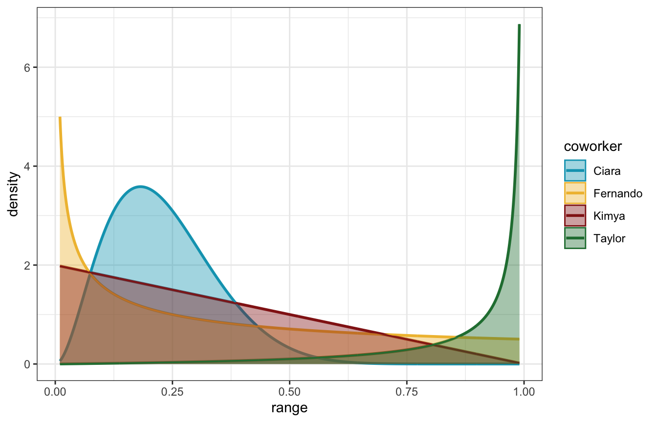

Kimya is relatively uncertain, but leaning towards believing that π is low
Fernando puts heavy weight on very low probabilities of π—moreso than Kimya
Ciara believes that π is clustered around 20%, and no higher than 50%
Taylor is the most optimistic, believing that π is exceptionally high (like 90+%)

4.5 & 4.6: Simulating and identifying the posterior

Chad peruses the shop’s website. On 3 of the past 7 days, they were still open at 2 p.m.. Complete the following for each of Chad’s coworkers:

simulate their posterior model;

create a histogram for the simulated posterior; and

use the simulation to approximate the posterior mean value of π

and

Complete the following for each of Chad’s coworkers:

identify the exact posterior model of π;

calculate the exact posterior mean of π; and

compare these to the simulation results in the previous exercise.

Ciara only

\[ \begin{aligned} (Y = 3) \mid \pi &= \operatorname{Binomial}(7, \pi) \\ \pi &\sim \operatorname{Beta}(3, 10) \end{aligned} \]

The Bayes Rules simulation approach is to simulate all the possibly likelihoods (here 0–7 / 7) and then filter to just choose one (3)

pi_ciara <- tibble(pi = rbeta(10000, 3, 10)) %>% 
  mutate(y = rbinom(10000, size = 7, prob = pi))

ggplot(pi_ciara, aes(x = pi, y = y)) +
  geom_point(aes(color = (y == 3)))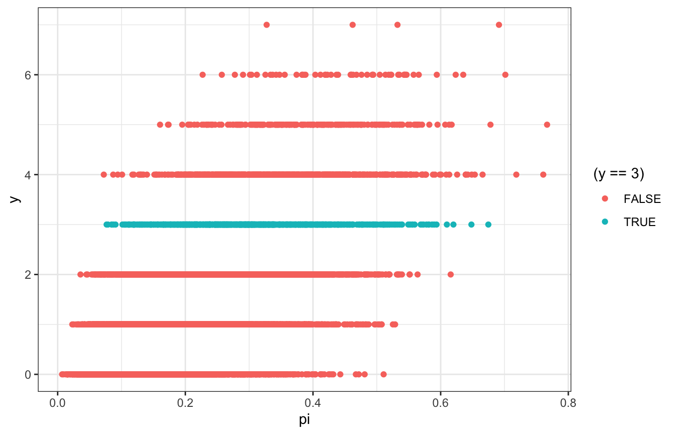

pi_ciara %>% 
  filter(y == 3) %>% 
  summarize(across(pi, lst(mean, median)))
## # A tibble: 1 × 2
##   pi_mean pi_median
##     <dbl>     <dbl>
## 1   0.302     0.296

pi_ciara %>% 
  filter(y == 3) %>% 
  ggplot(aes(x = pi)) +
  geom_density()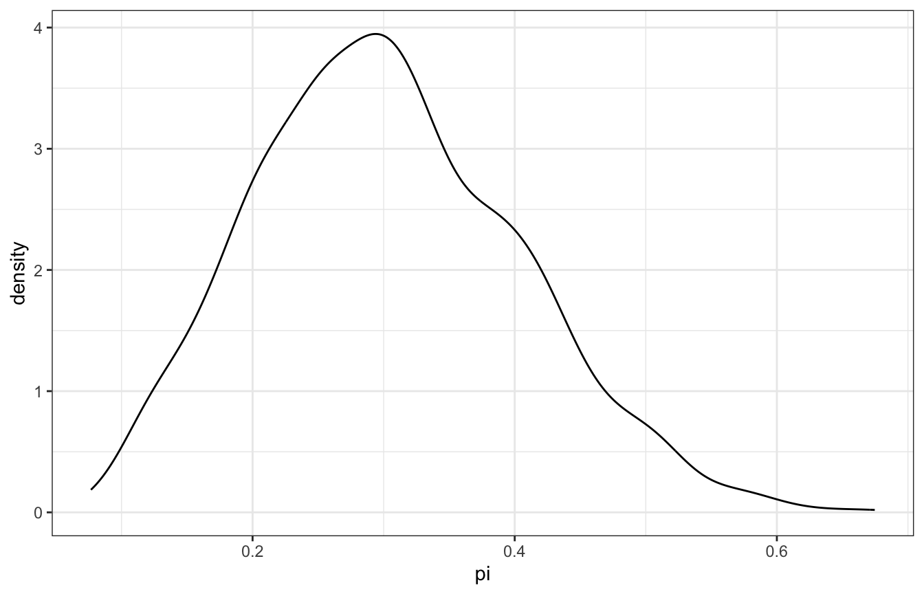

pi_grid <- tibble(pi_grid = seq(0, 1, length.out = 1001)) %>%
  mutate(prior_beta = dbeta(pi_grid, 3, 10)) %>% 
  mutate(likelihood = dbinom(3, size = 7, prob = pi_grid)) %>% 
  mutate(posterior = (likelihood * prior_beta) / sum(likelihood * prior_beta))

pi_samples <- pi_grid %>% 
  slice_sample(n = 10000, weight_by = posterior, replace = TRUE)

pi_samples %>% 
  summarize(across(pi_grid, lst(mean, median)))
## # A tibble: 1 × 2
##   pi_grid_mean pi_grid_median
##          <dbl>          <dbl>
## 1        0.301          0.295

ggplot(pi_samples, aes(x = pi_grid)) +
  geom_density()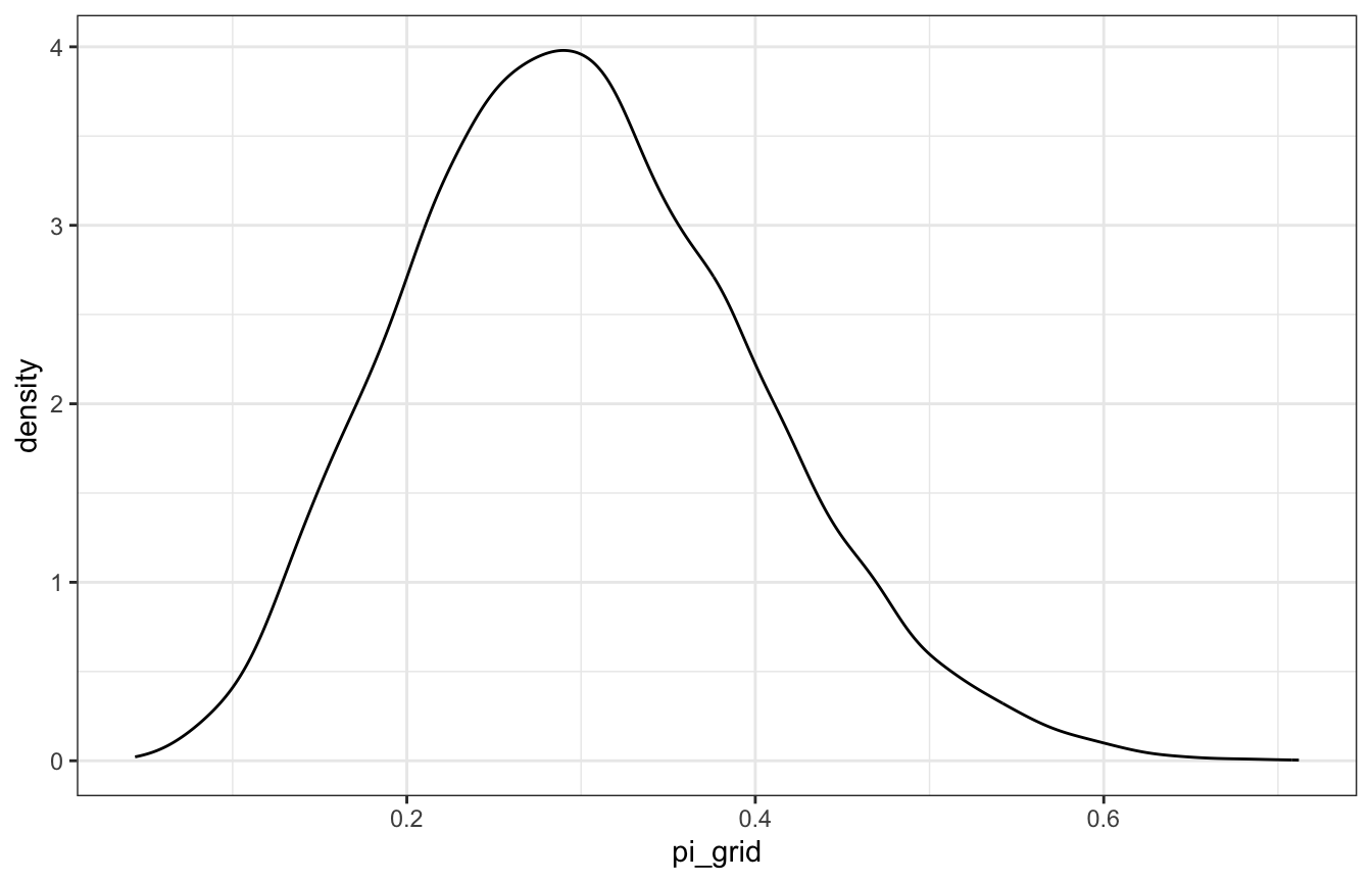

model_pi <- brm(
  bf(days_open | trials(weekdays) ~ 0 + Intercept),
  data = list(days_open = 3, weekdays = 7),
  family = binomial(link = "identity"),
  prior(beta(3, 10), class = b, lb = 0, ub = 1),
  iter = 5000, warmup = 1000, seed = BAYES_SEED,
  backend = "rstan", cores = 4
)
## Compiling Stan program...
## Start sampling

model_pi %>% 
  spread_draws(b_Intercept) %>%
  summarize(across(b_Intercept, lst(mean, median, hdci = ~median_hdci(., width = 0.89)))) %>% 
  unnest(b_Intercept_hdci)
## # A tibble: 1 × 8
##   b_Intercept_mean b_Intercept_median     y  ymin  ymax .width .point .interval
##              <dbl>              <dbl> <dbl> <dbl> <dbl>  <dbl> <chr>  <chr>    
## 1            0.298              0.292 0.292 0.110 0.493   0.95 median hdci

model_pi %>% 
  gather_draws(b_Intercept) %>% 
  ggplot(aes(x = .value)) +
  geom_density(aes(fill = "Posterior"), color = NA, alpha = 0.75) +
  stat_function(geom = "area", fun = ~dbeta(., 3, 10), aes(fill = "Beta(3, 10) prior"), alpha = 0.75) +
  scale_fill_manual(values = clrs[5:6]) +
  xlim(c(0, 1))

pi_stan.stan:

// Things coming in from R
data {
  int<lower=0> total_days;  // Possible days open (corresponds to binomial trials)
  int<lower=0> days_open;  // Outcome variable
}

// Things to estimate
parameters {
  real<lower=0, upper=1> pi;  // Probability the store is open
}

// Models and distributions
model {
  // Prior
  pi ~ beta(3, 10);
  
  // Likelihood
  days_open ~ binomial(total_days, pi);
  
  // Internally, these ~ formulas really look like this:
  //   target += beta_lpdf(pi | 3, 10);
  //   target += binomial_lpmf(days_open | total_days, pi);
  // The ~ notation is a lot nicer and maps onto the notation more directly
}

model_stan <- rstan::sampling(
  pi_stan,
  data = list(days_open = 3, total_days = 7),
  iter = 5000, warmup = 1000, seed = BAYES_SEED, chains = 4
)

model_stan %>% 
  spread_draws(pi) %>% 
  summarize(across(pi, lst(mean, median)))
## # A tibble: 1 × 2
##   pi_mean pi_median
##     <dbl>     <dbl>
## 1   0.298     0.292

model_stan %>% 
  spread_draws(pi) %>% 
  ggplot(aes(x = pi)) +
  stat_halfeye()
## Warning: Using the `size` aesthietic with geom_segment was deprecated in ggplot2 3.4.0.
## ℹ Please use the `linewidth` aesthetic instead.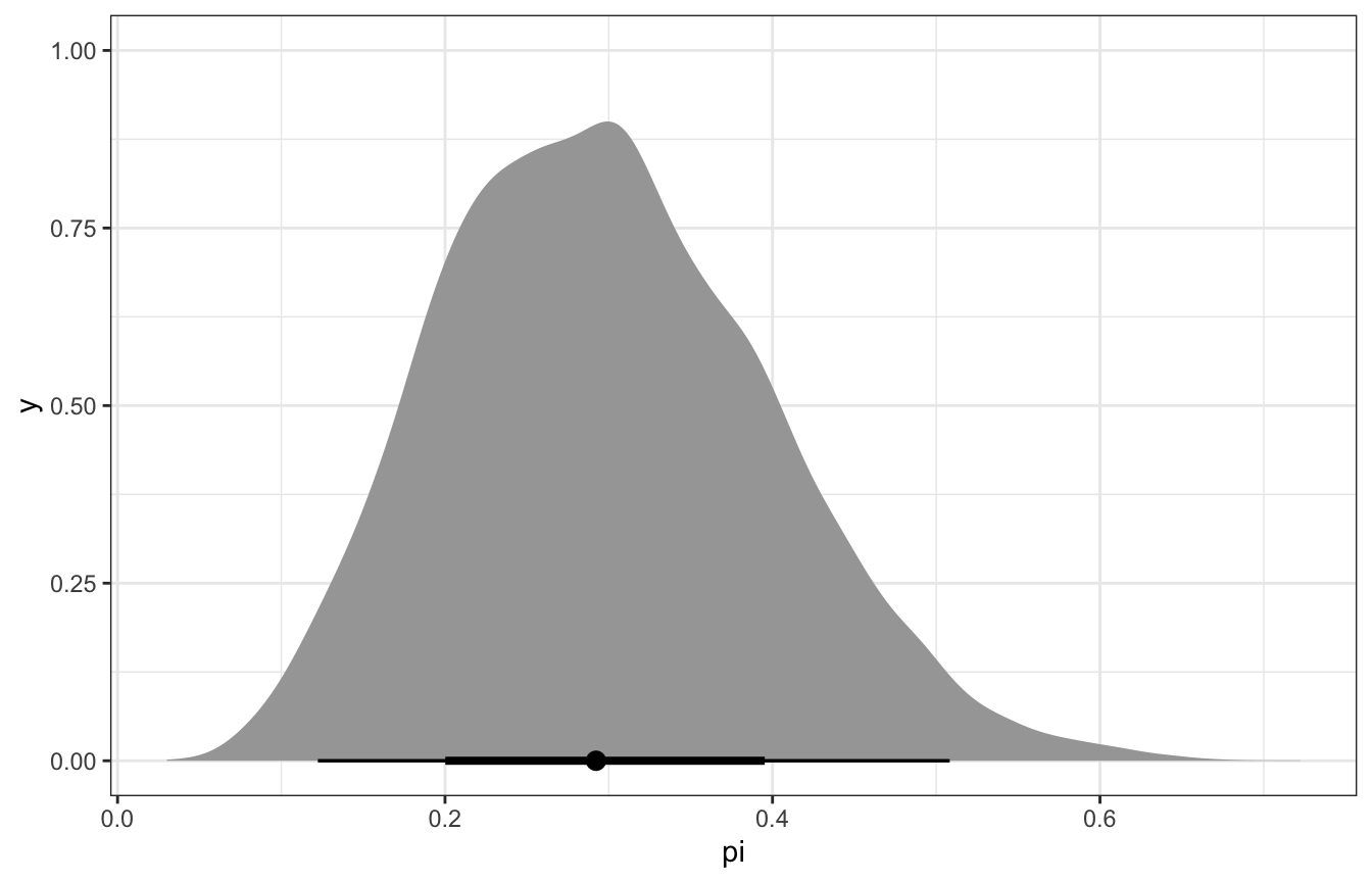

From equation 3.10 in Bayes Rules!:

\[ \begin{aligned} \pi \mid (Y = y) &\sim \operatorname{Beta}(\alpha + y, \quad \beta + n - y) \\ \pi \mid (Y = 3) &\sim \operatorname{Beta}(3 + 3, \quad 10 + 7 - 3) \\ &\sim \operatorname{Beta}(6, 14) \end{aligned} \]

ggplot() +
  geom_function(fun = ~dbeta(., 6, 14))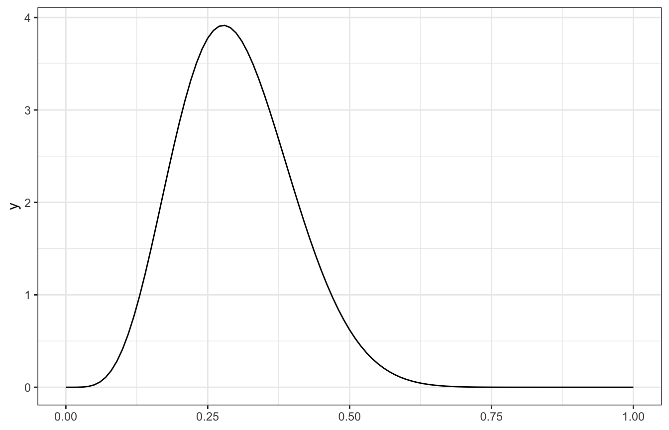

And from equation 3.11 in Bayes Rules!:

\[ \begin{aligned} E(\pi \mid Y = y) &= \frac{\alpha + y}{\alpha + \beta + n} \\ E(\pi \mid Y = 3) &= \frac{3 + 3}{3 + 10 + 7} \\ &= \frac{6}{20} = 0.3 \\ \end{aligned} \]

\[ \begin{aligned} \operatorname{Mode}(\pi \mid Y = y) &= \frac{\alpha + y - 1}{\alpha + \beta + n - 2} \\ \operatorname{Mode}(\pi \mid Y = 3) &= \frac{3 + 3 - 1}{3 + 10 + 7 - 2} \\ &= \frac{5}{18} = 0.27\bar{7} \\ \end{aligned} \]

\[ \begin{aligned} \operatorname{Var}(\pi \mid Y = y) &= \frac{(\alpha + y)~(\beta + n - y)}{(\alpha + \beta + n)^2~(\alpha + \beta + n + 1)} \\ \operatorname{Var}(\pi \mid Y = 3) &= \frac{(3 + 3)~(10 + 7 - 3)}{(3 + 10 + 7)^2~(3 + 10 + 7 + 1)} \\ &= \frac{6 \times 14}{20^2 \times 21} = \frac{84}{8,400} = 0.01 \\ \operatorname{SD}(\pi \mid Y = 3) &= \sqrt{0.01} = 0.1 \end{aligned} \]

Verify using summarize_beta_binomial():

summarize_beta_binomial(alpha = 3, beta = 10, y = 3, n = 7)
##       model alpha beta      mean      mode        var        sd
## 1     prior     3   10 0.2307692 0.1818182 0.01267963 0.1126039
## 2 posterior     6   14 0.3000000 0.2777778 0.01000000 0.1000000

All four coworkers

(sans raw Stan; brms is fine and great for this anyway)

# Clean this table of coworkers up a bit
priors_clean <- worker_prior_densities %>% 
  select(coworker, prior, shape1, shape2)

priors_clean %>% 
  knitr::kable()

coworker	prior	shape1	shape2
Kimya	Beta(1, 2)	1.0	2.0
Fernando	Beta(0.5, 1)	0.5	1.0
Ciara	Beta(3, 10)	3.0	10.0
Taylor	Beta(2, 0.1)	2.0	0.1

br_simulation_pi <- priors_clean %>% 
  mutate(pi_sim = map2(shape1, shape2, ~{
    tibble(pi = rbeta(10000, .x, .y)) %>% 
      mutate(y = rbinom(10000, size = 7, prob = pi))
  }))

br_simulation_pi %>% 
  unnest(pi_sim) %>% 
  ggplot(aes(x = pi, y = y)) +
  geom_point(aes(color = (y == 3))) +
  facet_wrap(vars(coworker))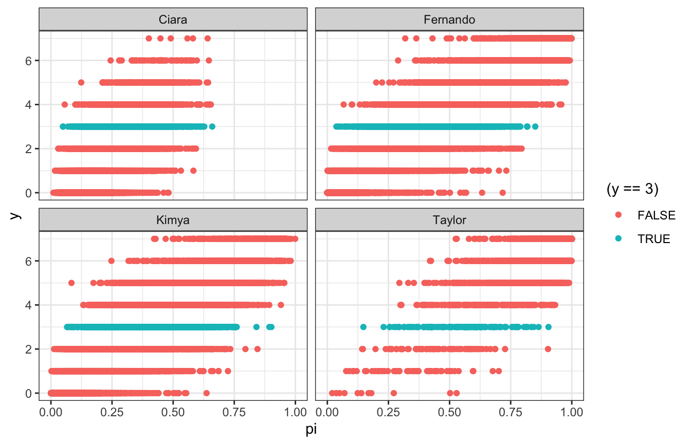

br_simulation_pi %>% 
  unnest(pi_sim) %>% 
  filter(y == 3) %>% 
  group_by(coworker) %>% 
  summarize(across(pi, lst(mean, median)))
## # A tibble: 4 × 3
##   coworker pi_mean pi_median
##   <chr>      <dbl>     <dbl>
## 1 Ciara      0.305     0.297
## 2 Fernando   0.416     0.414
## 3 Kimya      0.400     0.391
## 4 Taylor     0.545     0.564

br_simulation_pi %>% 
  unnest(pi_sim) %>% 
  filter(y == 3) %>% 
  ggplot(aes(x = pi, fill = coworker, color = coworker)) +
  geom_density(size = 1, alpha = 0.4) +
  scale_fill_manual(values = clrs[c(1, 2, 3, 5)]) +
  scale_color_manual(values = clrs[c(1, 2, 3, 5)])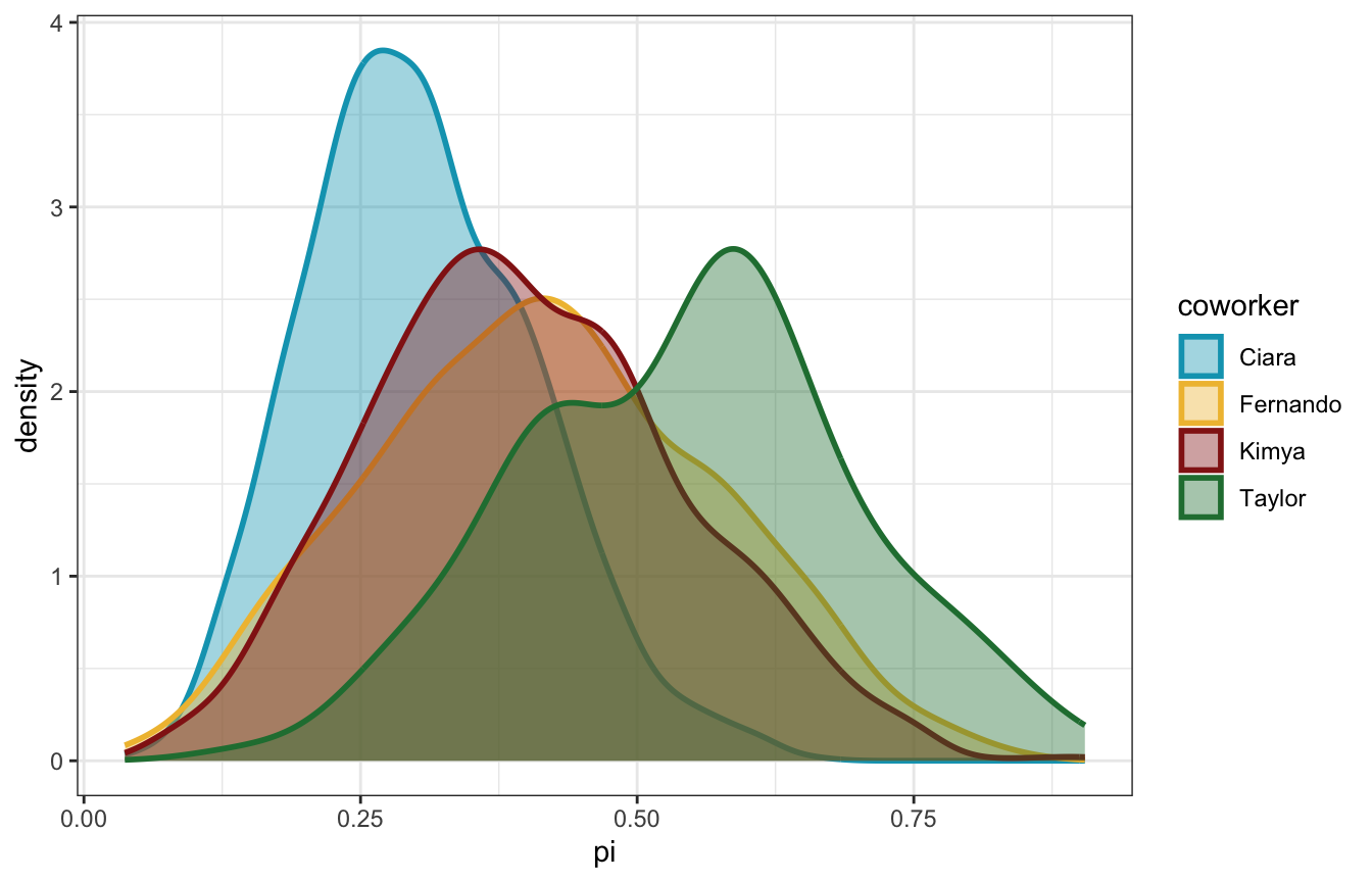

Cool cool. Fernando and Kimya’s flatter priors end up leading to posteriors of ≈40%. Taylor’s extreme optimism leads to a posterior mean of 57%! Ciara’s more reasonable range leads to a posterior of 30%.

grid_simulation_pi <- priors_clean %>% 
  mutate(pi_grid = list(seq(0.01, 0.99, length.out = 1001))) %>% 
  mutate(prior_beta = pmap(list(pi_grid, shape1, shape2), ~{
    dbeta(..1, ..2, ..3)
  })) %>% 
  mutate(likelihood = map(pi_grid, ~{
    dbinom(3, size = 7, prob = .x)
  })) %>% 
  mutate(posterior = map2(prior_beta, likelihood, ~{
    (.y * .x) / sum(.y * .x)
  })) 

grid_simulation_samples <- grid_simulation_pi %>% 
  unnest(c(pi_grid, posterior)) %>% 
  group_by(coworker) %>% 
  slice_sample(n = 10000, weight_by = posterior, replace = TRUE)

grid_simulation_samples %>% 
  group_by(coworker) %>% 
  summarize(across(pi_grid, lst(mean, median)))
## # A tibble: 4 × 3
##   coworker pi_grid_mean pi_grid_median
##   <chr>           <dbl>          <dbl>
## 1 Ciara           0.300          0.294
## 2 Fernando        0.412          0.405
## 3 Kimya           0.399          0.394
## 4 Taylor          0.550          0.555

grid_simulation_samples %>% 
  ggplot(aes(x = pi_grid, fill = coworker, color = coworker)) +
  geom_density(size = 1, alpha = 0.4) +
  scale_fill_manual(values = clrs[c(1, 2, 3, 5)]) +
  scale_color_manual(values = clrs[c(1, 2, 3, 5)])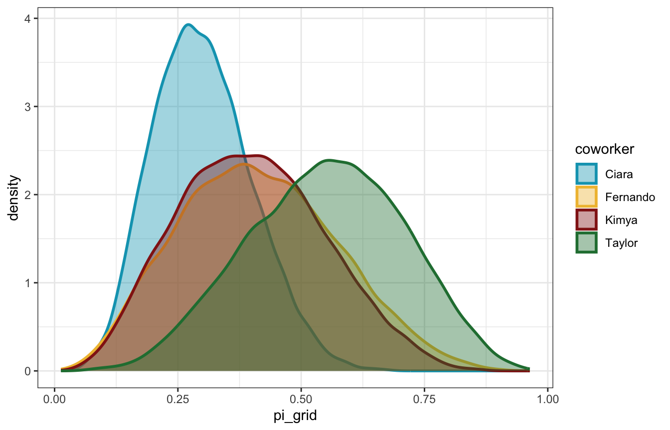

brms_pi <- priors_clean %>% 
  mutate(stan_prior = map2(shape1, shape2, ~{
    prior_string(glue::glue("beta({.x}, {.y})"), class = "b", lb = 0, ub = 1)
  })) %>% 
  mutate(model = map(stan_prior, ~{
    brm(
      bf(days_open | trials(weekdays) ~ 0 + Intercept),
      data = list(days_open = 3, weekdays = 7),
      family = binomial(link = "identity"),
      prior = .x,
      iter = 5000, warmup = 1000, seed = BAYES_SEED,
      backend = "rstan", cores = 4
    )
  }))
## Compiling Stan program...
## Start sampling
## Compiling Stan program...
## Start sampling
## Compiling Stan program...
## Start sampling
## Compiling Stan program...
## Start sampling

brms_pi %>% 
  mutate(draws = map(model, ~spread_draws(., b_Intercept))) %>% 
  unnest(draws) %>% 
  group_by(coworker) %>% 
  summarize(across(b_Intercept, lst(mean, median, hdci = ~median_hdci(., width = 0.89)))) %>% 
  unnest(b_Intercept_hdci)
## # A tibble: 4 × 9
##   coworker b_Intercept_mean b_Intercep…¹     y  ymin  ymax .width .point .inte…²
##   <chr>               <dbl>        <dbl> <dbl> <dbl> <dbl>  <dbl> <chr>  <chr>  
## 1 Ciara               0.298        0.292 0.292 0.110 0.493   0.95 median hdci   
## 2 Fernando            0.411        0.403 0.403 0.125 0.726   0.95 median hdci   
## 3 Kimya               0.399        0.392 0.392 0.130 0.693   0.95 median hdci   
## 4 Taylor              0.547        0.552 0.552 0.258 0.850   0.95 median hdci   
## # … with abbreviated variable names ¹b_Intercept_median, ².interval

brms_pi %>% 
  mutate(draws = map(model, ~gather_draws(., b_Intercept))) %>% 
  unnest(draws) %>% 
  ggplot(aes(x = .value, fill = coworker)) +
  stat_halfeye(alpha = 0.4) +
  scale_fill_manual(values = clrs[c(1, 2, 3, 5)])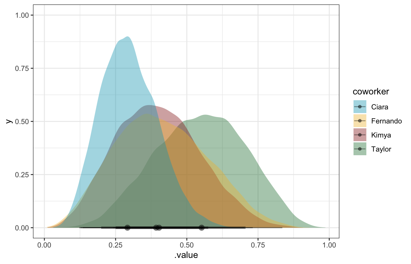

lik_y <- 3
lik_n <- 7

posteriors_manual <- priors_clean %>% 
  mutate(posterior_shape1 = shape1 + lik_y,
         posterior_shape2 = shape2 + lik_n - lik_y)

posteriors_manual %>% 
  mutate(posterior = glue::glue("Beta({posterior_shape1}, {posterior_shape2})")) %>% 
  select(coworker, prior, posterior) %>% 
  knitr::kable()

coworker	prior	posterior
Kimya	Beta(1, 2)	Beta(4, 6)
Fernando	Beta(0.5, 1)	Beta(3.5, 5)
Ciara	Beta(3, 10)	Beta(6, 14)
Taylor	Beta(2, 0.1)	Beta(5, 4.1)

posteriors_manual_plot <- posteriors_manual %>% 
  mutate(range = list(seq(0.01, 0.99, length.out = 1001))) %>% 
  mutate(density = pmap(list(range, posterior_shape1, posterior_shape2), ~dbeta(..1, ..2, ..3)))

posteriors_manual_plot %>% 
  unnest(c(range, density)) %>% 
  ggplot(aes(x = range, y = density, fill = coworker, color = coworker)) +
  geom_line(size = 1) +
  geom_area(position = position_identity(), alpha = 0.4) +
  scale_fill_manual(values = clrs[c(1, 2, 3, 5)]) +
  scale_color_manual(values = clrs[c(1, 2, 3, 5)])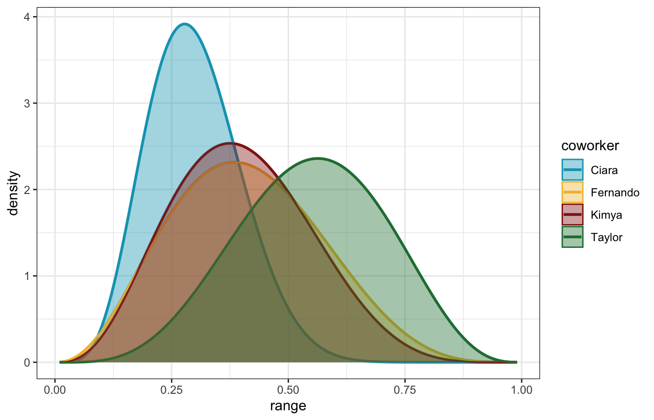

posteriors_manual_summary <- posteriors_manual %>% 
  group_by(coworker) %>% 
  summarize(summary = map2(shape1, shape2, ~{
    summarize_beta_binomial(alpha = .x, beta = .y, y = lik_y, n = lik_n)
  })) %>% 
  unnest(summary) 

posteriors_manual_summary %>% 
  select(-coworker) %>% 
  kableExtra::kbl(digits = 3) %>% 
  kableExtra::pack_rows(index = table(posteriors_manual_summary$coworker)) %>% 
  kableExtra::kable_styling()

model	alpha	beta	mean	mode	var	sd
Ciara
prior	3.0	10.0	0.231	0.182	0.013	0.113
posterior	6.0	14.0	0.300	0.278	0.010	0.100
Fernando
prior	0.5	1.0	0.333	1.000	0.089	0.298
posterior	3.5	5.0	0.412	0.385	0.025	0.160
Kimya
prior	1.0	2.0	0.333	0.000	0.056	0.236
posterior	4.0	6.0	0.400	0.375	0.022	0.148
Taylor
prior	2.0	0.1	0.952	1.000	0.015	0.121
posterior	5.0	4.1	0.549	0.563	0.025	0.157