Video #7 code

Overfitting

Published

October 5, 2022

library(tidyverse)
library(brms)
library(loo)
library(tidybayes)

# Plot stuff
clrs <- MetBrewer::met.brewer("Lakota", 6)
theme_set(theme_bw())

# Seed stuff
set.seed(1234)
BAYES_SEED <- 1234

data(WaffleDivorce, package = "rethinking")

WaffleDivorce <- WaffleDivorce %>% 
  mutate(across(c(Marriage, Divorce, MedianAgeMarriage), ~scale(.), .names = "{col}_scaled")) %>% 
  mutate(across(c(Marriage, Divorce, MedianAgeMarriage), ~as.numeric(scale(.)), .names = "{col}_z"))

Finding outliers with PSIS and WAIC

ggplot(WaffleDivorce, aes(x = MedianAgeMarriage_z, y = Divorce_z)) +
  geom_point(aes(color = Loc %in% c("ME", "ID")), size = 2) +
  geom_text(data = filter(WaffleDivorce, Loc %in% c("ME", "ID")), 
            aes(label = Location), hjust = -0.25) +
  scale_color_manual(values = c("grey40", clrs[4]), guide = "none") +
  labs(x = "Age at marriage (standardized)", y = "Divorce rate (standardized)")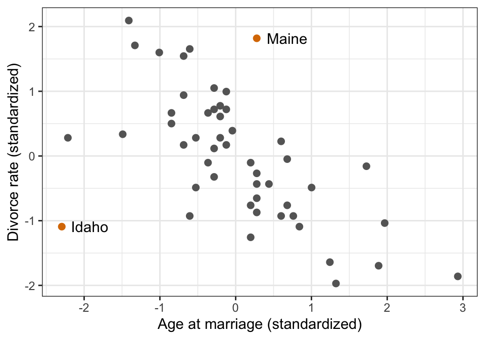

Run a model:

priors <- c(prior(normal(0, 0.2), class = Intercept),
            prior(normal(0, 0.5), class = b, coef = "Marriage_z"),
            prior(normal(0, 0.5), class = b, coef = "MedianAgeMarriage_z"),
            prior(exponential(1), class = sigma))

marriage_divorce_normal <- brm(
  bf(Divorce_z ~ Marriage_z + MedianAgeMarriage_z),
  data = WaffleDivorce,
  family = gaussian(),
  prior = priors,
  chains = 4, cores = 4, seed = BAYES_SEED, 
  backend = "cmdstanr", refresh = 0
)
## Start sampling

Check the LOO stats. One value is fairly influential with k > 0.5, but the others are okay:

loo(marriage_divorce_normal)
## 
## Computed from 4000 by 50 log-likelihood matrix
## 
##          Estimate   SE
## elpd_loo    -63.8  6.4
## p_loo         4.8  1.9
## looic       127.7 12.8
## ------
## Monte Carlo SE of elpd_loo is 0.1.
## 
## Pareto k diagnostic values:
##                          Count Pct.    Min. n_eff
## (-Inf, 0.5]   (good)     49    98.0%   688       
##  (0.5, 0.7]   (ok)        1     2.0%   176       
##    (0.7, 1]   (bad)       0     0.0%   <NA>      
##    (1, Inf)   (very bad)  0     0.0%   <NA>      
## 
## All Pareto k estimates are ok (k < 0.7).
## See help('pareto-k-diagnostic') for details.

Which observation has the high PSIS k value?

loo(marriage_divorce_normal) |> 
  pareto_k_ids()
## [1] 13

Row 13! Which is…

WaffleDivorce |> 
  slice(13) |> 
  select(Location)
##   Location
## 1    Idaho

Idaho.

How big is the actual k value?

loo(marriage_divorce_normal) |> 
  pareto_k_values() |> 
  pluck(13)
## [1] 0.6065822

We can embed these diagnostics into the brms object with add_criterion():

marriage_divorce_normal <- add_criterion(marriage_divorce_normal, criterion = "loo")
marriage_divorce_normal <- add_criterion(marriage_divorce_normal, criterion = "waic")
## Warning: 
## 2 (4.0%) p_waic estimates greater than 0.4. We recommend trying loo instead.

And that lets us access things in deeply nested lists, like the 13th Pareto k value:

marriage_divorce_normal$criteria$loo$diagnostics$pareto_k[13]
## [1] 0.6065822

Neat. Now we can plot these k values and WAIC values and recreate Figure 7.10 from the book and from 1:03:00 in lecture video 7.

tibble(psis = marriage_divorce_normal$criteria$loo$diagnostics$pareto_k,
       p_waic = marriage_divorce_normal$criteria$waic$pointwise[, "p_waic"],
       Location = pull(WaffleDivorce, Location),
       Loc = pull(WaffleDivorce, Loc)) %>%
  ggplot(aes(x = psis, y = p_waic)) +
  geom_point(aes(color = Loc %in% c("ME", "ID")), size = 2) +
  geom_text(data = . %>% filter(Loc %in% c("ME", "ID")), 
            aes(label = Location), hjust = 1.25) +
  geom_vline(xintercept = 0.5, linetype = 32) +
  scale_color_manual(values = c("grey40", clrs[4]), guide = "none") +
  labs(x = "PSIS Pareto k", y = "WAIC penalty")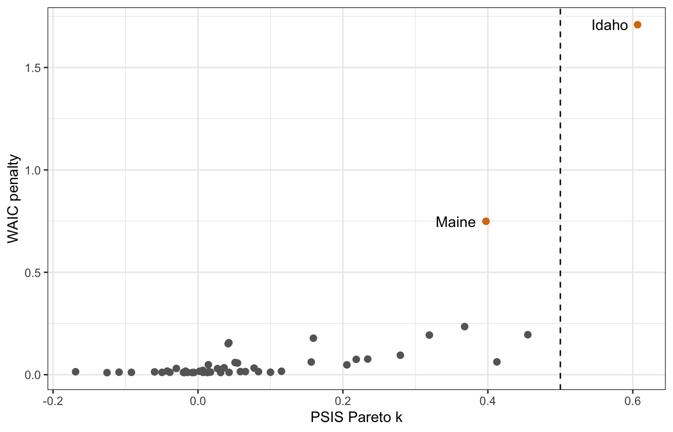

Robust regression

We can do robust regression with family = student(), which has thicker tails and expects larger values out in the tails

priors <- c(prior(normal(0, 0.2), class = Intercept),
            prior(normal(0, 0.5), class = b, coef = "Marriage_z"),
            prior(normal(0, 0.5), class = b, coef = "MedianAgeMarriage_z"),
            prior(exponential(1), class = sigma))

marriage_divorce_student <- brm(
  bf(Divorce_z ~ Marriage_z + MedianAgeMarriage_z,
     nu = 2),  # Tail thickness
  data = WaffleDivorce,
  family = student(),
  prior = priors,
  chains = 4, cores = 4, seed = BAYES_SEED, 
  backend = "cmdstanr", refresh = 0
)
## Start sampling

Add penalty statistics to the model object:

marriage_divorce_student <- add_criterion(marriage_divorce_student, criterion = c("loo", "waic"))
## Warning: 
## 2 (4.0%) p_waic estimates greater than 0.4. We recommend trying loo instead.

plot_data <- tibble(psis = marriage_divorce_student$criteria$loo$diagnostics$pareto_k,
                    p_waic = marriage_divorce_student$criteria$waic$pointwise[, "p_waic"],
                    Location = pull(WaffleDivorce, Location),
                    Loc = pull(WaffleDivorce, Loc)) 
plot_data %>%
  ggplot(aes(x = psis, y = p_waic)) +
  geom_point(aes(color = Loc %in% c("ME", "ID")), size = 2) +
  geom_text(data = . %>% filter(Loc %in% c("ME", "ID")), 
            aes(label = Location), hjust = 1.25) +
  geom_vline(xintercept = 0.5, linetype = 32) +
  scale_color_manual(values = c("grey40", clrs[4]), guide = "none") +
  labs(x = "PSIS Pareto k", y = "WAIC penalty")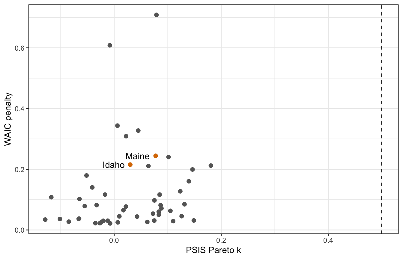

Hey hey, Idaho and Maine have much lower PSIS k values now. There are some weird observations with really high WAIC values for some reason:

plot_data |> 
  arrange(desc(p_waic))
## # A tibble: 50 × 4
##        psis p_waic Location     Loc  
##       <dbl>  <dbl> <fct>        <fct>
##  1  0.0790   0.709 Wyoming      WY   
##  2 -0.00816  0.608 Utah         UT   
##  3  0.00618  0.344 Arkansas     AR   
##  4  0.0451   0.327 North Dakota ND   
##  5  0.0223   0.309 Alaska       AK   
##  6  0.0775   0.244 Maine        ME   
##  7  0.102    0.240 Rhode Island RI   
##  8  0.0301   0.215 Idaho        ID   
##  9  0.181    0.212 Minnesota    MN   
## 10  0.0640   0.211 New Jersey   NJ   
## # … with 40 more rows

Wyoming and Utah! Why? I don’t know :(

Compare the models

We can compare the two models’ LOO statistics:

loo_compare(marriage_divorce_normal, marriage_divorce_student, criterion = "loo")
##                          elpd_diff se_diff
## marriage_divorce_normal   0.0       0.0   
## marriage_divorce_student -2.5       3.0
loo_compare(marriage_divorce_normal, marriage_divorce_student, criterion = "waic")
##                          elpd_diff se_diff
## marriage_divorce_normal   0.0       0.0   
## marriage_divorce_student -2.7       2.9

The normal model has the higher ELPD score (so it’s better), but the standard error is huge and makes the models indistinguishable (so it’s not necessarily better)

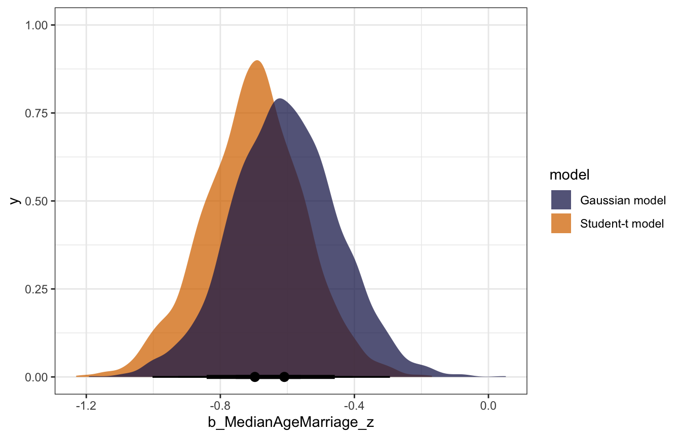
We can also compare the posterior distributions for the effect of age on marriage. The coefficient for age in the Student-t model is more negative and more precise. Idaho was making the normal model too skeptical and too surprised; the Student-t model was less surprised by it.

normal_coefs <- marriage_divorce_normal |> 
  spread_draws(b_MedianAgeMarriage_z) |> 
  mutate(model = "Gaussian model")

student_coefs <- marriage_divorce_student |> 
  spread_draws(b_MedianAgeMarriage_z) |> 
  mutate(model = "Student-t model")

bind_rows(normal_coefs, student_coefs) |> 
  ggplot(aes(x = b_MedianAgeMarriage_z, fill = model)) +
  stat_halfeye(slab_alpha = 0.75) +
  scale_fill_manual(values = c(clrs[6], clrs[4]))