Chapter 3 notes

Posteriors from grids

Published

September 2, 2022

library(tidyverse)
library(brms)
library(tidybayes)
library(patchwork)
library(posterior)
library(broom.mixed)

set.seed(1234)

Assuming 9 globe tosses, 6 are water:

W L W W W L W L W

Or in code:

tosses <- c("W", "L", "W", "W", "W", "L", "W", "L", "W")
table(tosses)
## tosses
## L W 
## 3 6

Given this data, what’s the proportion of water on the globe?

Make a list of all possible proportions, ranging from 0 to 1
Calculate the number of possible pathways to get to that proportion

Grid approximation

For each possible value of \(p\), compute the product \(\operatorname{Pr}(W, L \mid p) \times \operatorname{Pr}(p)\). The relative sizes of each of those products are the posterior probabilities.

Base R with Rethinking

Uniform flat prior

# List of possible explanations of p to consider
p_grid <- seq(from = 0, to = 1, length.out = 10000)
plot(p_grid, main = "Possible proportions (p)")
#

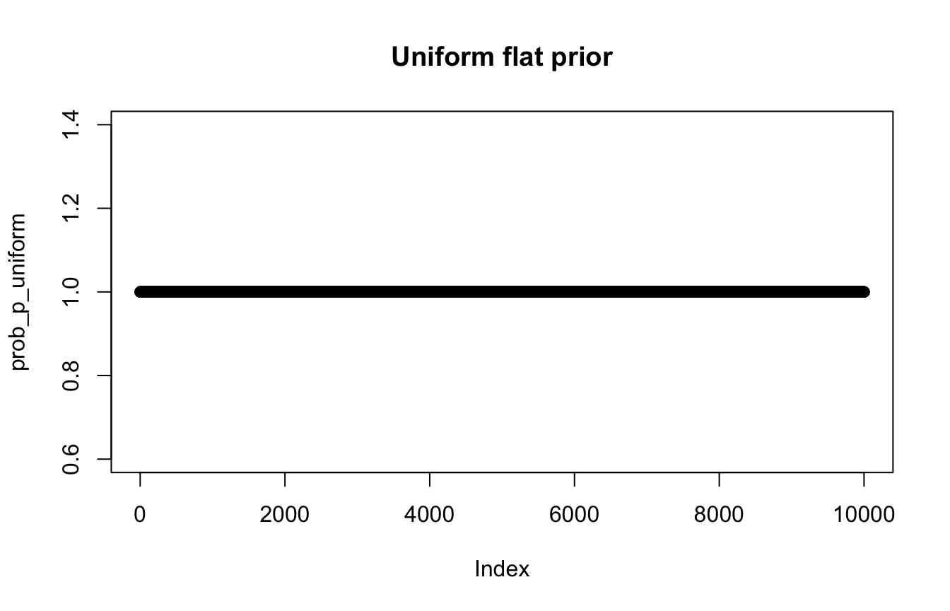
# Probability of each value of p
# Super vague uniform prior: just 1 at each possible p
prob_p_uniform <- rep(1, 10000)
plot(prob_p_uniform, main = "Uniform flat prior")
#

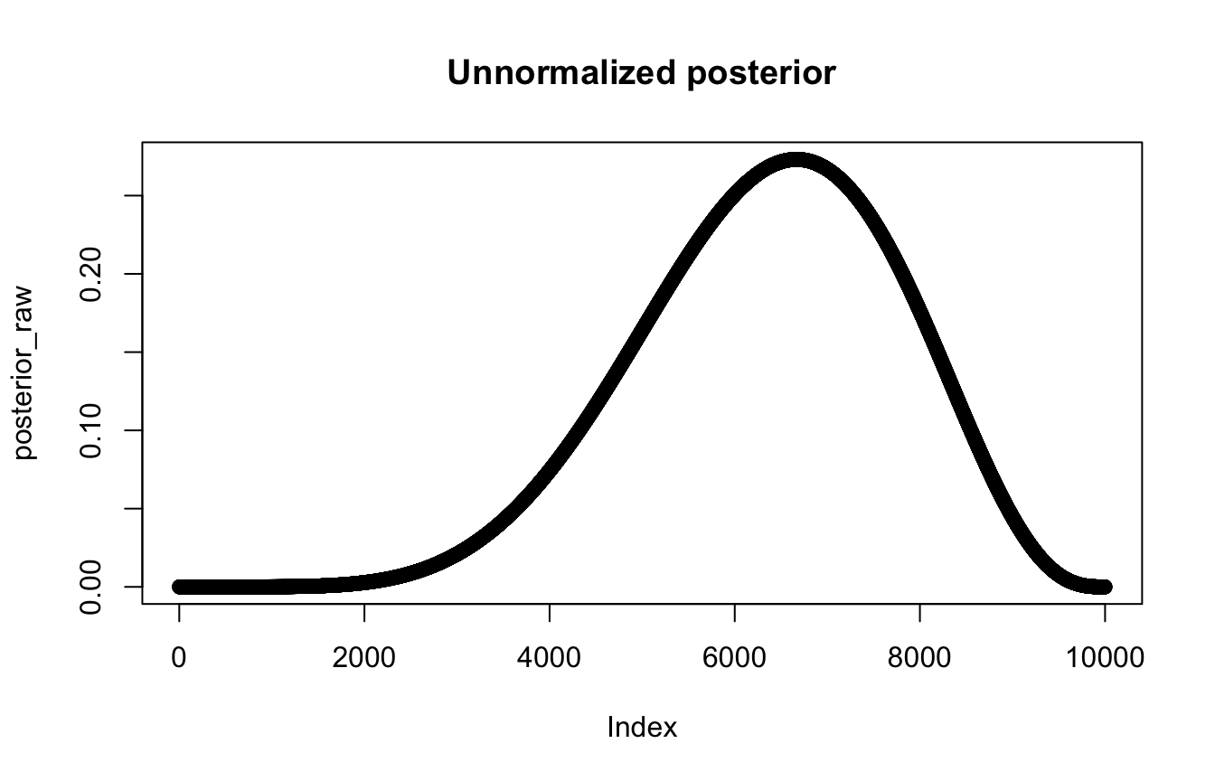
# Probability of each proportion, given 6/9 water draws
prob_data <- dbinom(6, size = 9, prob = p_grid)

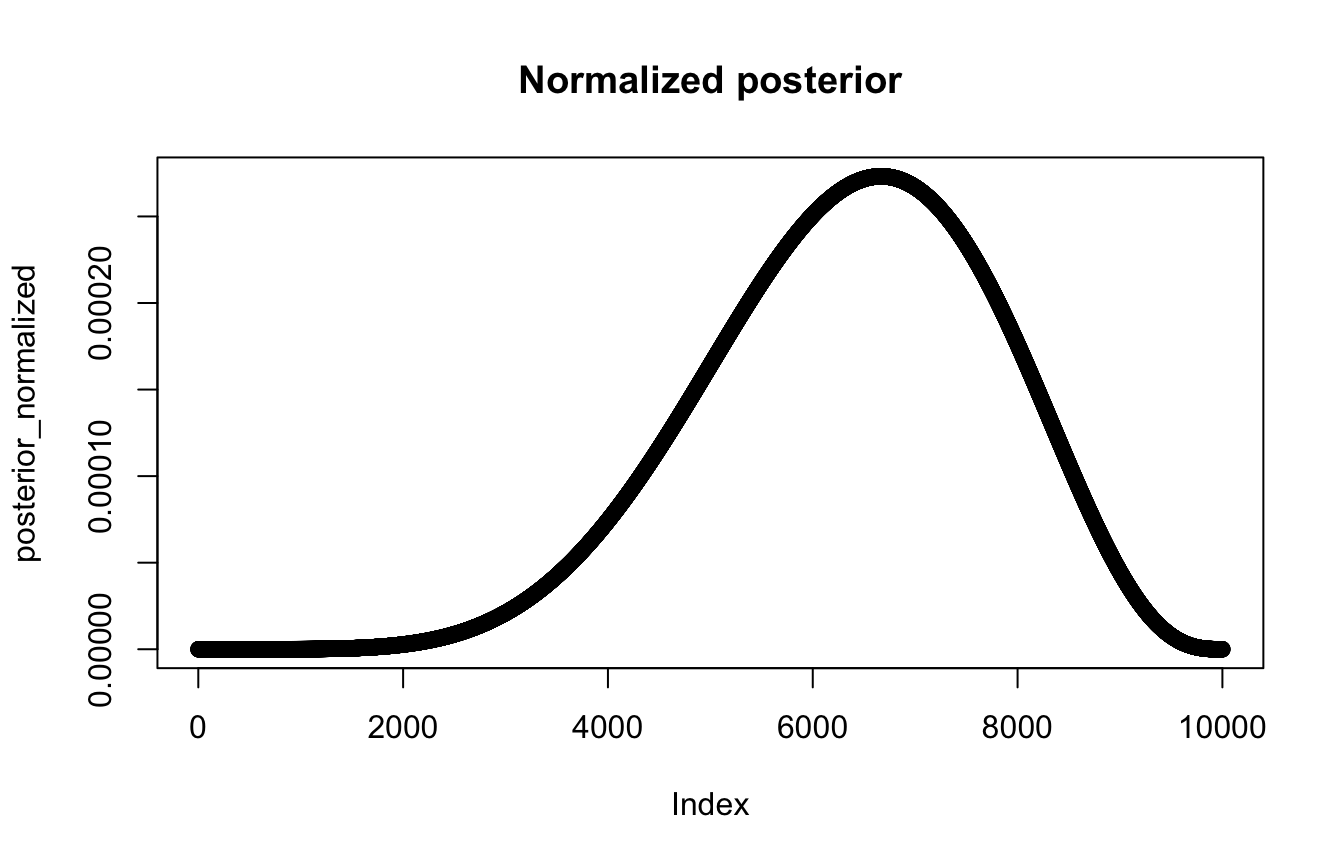
# Unnormalized posterior
posterior_raw <- prob_data * prob_p_uniform
plot(posterior_raw, main = "Unnormalized posterior")
#

# Normalized posterior that sums to 1
posterior_normalized <- posterior_raw / sum(posterior_raw)
plot(posterior_normalized, main = "Normalized posterior")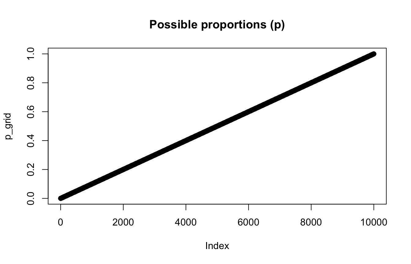

Beta prior

# Beta distribution with 3 / (3 + 1)
prob_p_beta <- dbeta(p_grid, shape1 = 3, shape2 = 1)
plot(prob_p_beta, main = "Beta(3, 1) prior")
#
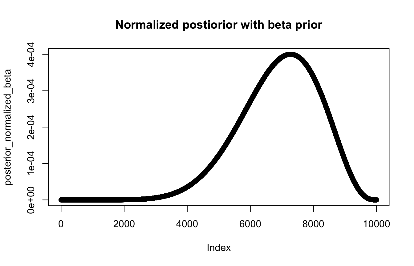
# Posterior that sums to 1
posterior_normalized_beta <- (prob_data * prob_p_beta) / sum(posterior_raw)
plot(posterior_normalized_beta, main = "Normalized postiorior with beta prior")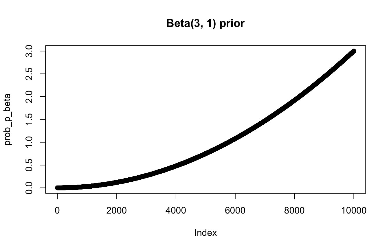

Tidyverse style from Solomon Kurz

globe_tossing <- tibble(p_grid = seq(from = 0, to = 1, length.out = 1001),
                        prior_uniform = 1) %>%  # prob_p_uniform from earlier
  mutate(prior_beta = dbeta(p_grid, shape1 = 3, shape2 = 1)) %>%  # prob_p_beta from earlier
  mutate(likelihood = dbinom(6, size = 9, prob = p_grid)) %>%   # prob_data from earlier
  mutate(posterior_uniform = (likelihood * prior_uniform) / sum(likelihood * prior_uniform),
         posterior_beta = (likelihood * prior_beta) / sum(likelihood * prior_beta))
globe_tossing
## # A tibble: 1,001 × 6
##    p_grid prior_uniform prior_beta likelihood posterior_uniform posterior_beta
##     <dbl>         <dbl>      <dbl>      <dbl>             <dbl>          <dbl>
##  1  0                 1  0           0                 0              0       
##  2  0.001             1  0.000003    8.37e-17          8.37e-19       1.97e-24
##  3  0.002             1  0.000012    5.34e-15          5.34e-17       5.04e-22
##  4  0.003             1  0.0000270   6.07e-14          6.07e-16       1.29e-20
##  5  0.004             1  0.000048    3.40e-13          3.40e-15       1.28e-19
##  6  0.005             1  0.000075    1.29e-12          1.29e-14       7.62e-19
##  7  0.006             1  0.000108    3.85e-12          3.85e-14       3.27e-18
##  8  0.007             1  0.000147    9.68e-12          9.68e-14       1.12e-17
##  9  0.008             1  0.000192    2.15e-11          2.15e-13       3.24e-17
## 10  0.009             1  0.000243    4.34e-11          4.34e-13       8.30e-17
## # … with 991 more rows

globe_tossing %>% 
  pivot_longer(starts_with("posterior")) %>% 
  ggplot(aes(x = p_grid, y = value, fill = name)) +
  geom_area(position = position_identity(), alpha = 0.5)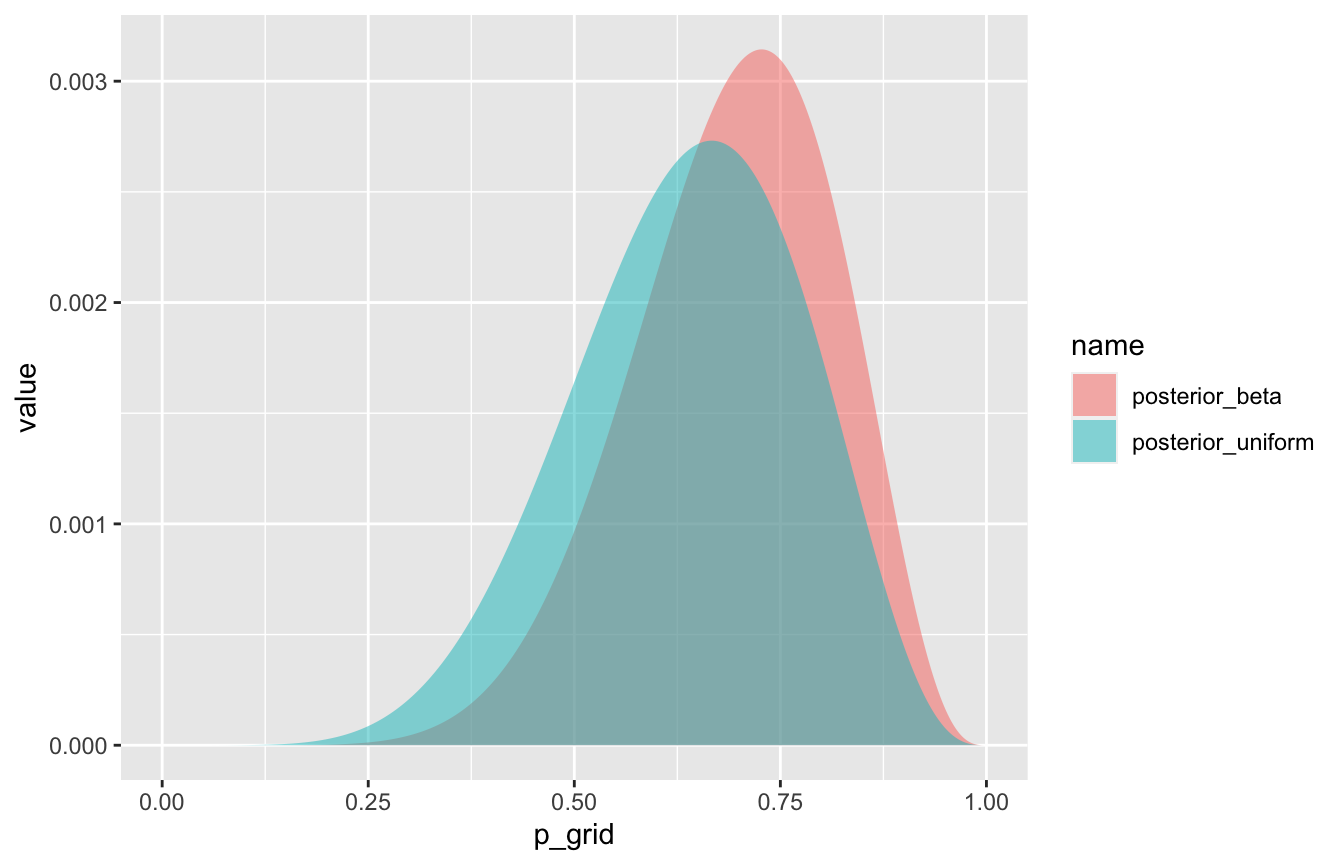

Working with the posterior

We now have a posterior! We typically can’t use the posterior alone. We have to average any inference across the entire posterior. This requires calculus, which is (1) hard, and (2) often impossible. So instead, we can use samples from the distribution and make inferences based on those.

3.2: Sampling to summarize

Here are 10,000 samples from the posterior (based on the uniform flat prior). These are the sampling distributions.

samples <- sample(p_grid, prob = posterior_normalized, size = 10000, replace = TRUE)
plot(samples, main = "10,000 posterior samples")
#

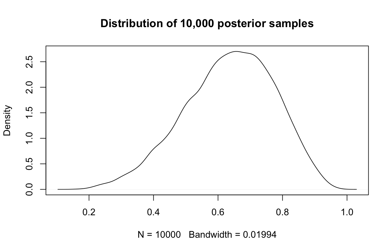
plot(density(samples), main = "Distribution of 10,000 posterior samples")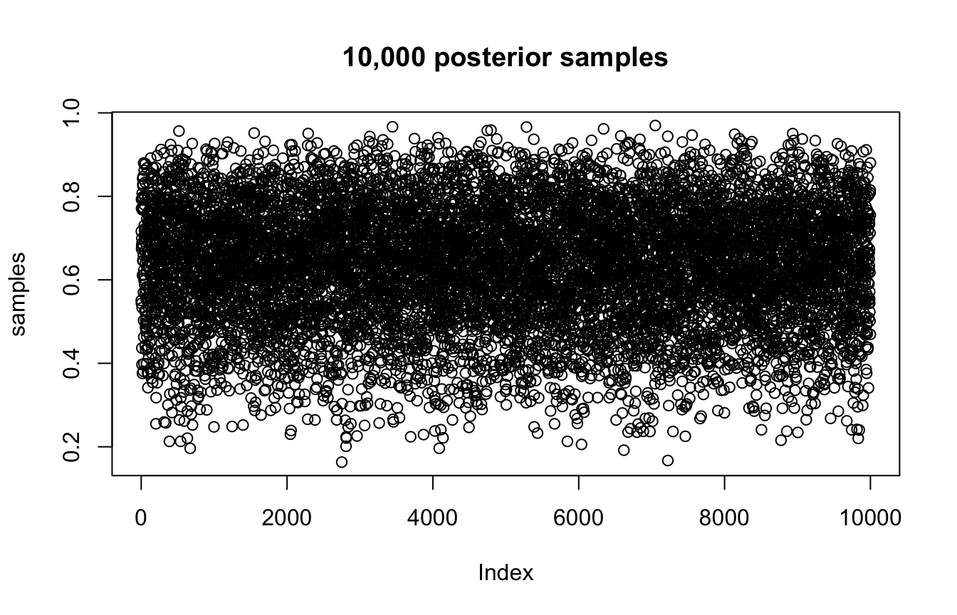

samples_tidy <- globe_tossing %>% 
  slice_sample(n = 10000, weight_by = posterior_uniform, replace = T)

What’s the probability that the proportion of water is less than 50%?

sum(samples < 0.5) / 10000
## [1] 0.1745

How much of the posterior is between 50% and 75%?

sum(samples > 0.5 & samples < 0.75) / 10000
## [1] 0.6037

What’s the probability that the proportion of water is less than 50%?

globe_tossing %>% 
  ggplot(aes(x = p_grid, y = posterior_uniform)) +
  geom_line() +
  geom_area(data = filter(globe_tossing, p_grid < 0.5))


samples_tidy %>% 
  count(p_grid < 0.5) %>% 
  mutate(probability = n / sum(n))
## # A tibble: 2 × 3
##   `p_grid < 0.5`     n probability
##   <lgl>          <int>       <dbl>
## 1 FALSE           8321       0.832
## 2 TRUE            1679       0.168

How much of the posterior is between 50% and 75%?

globe_tossing %>% 
  ggplot(aes(x = p_grid, y = posterior_uniform)) +
  geom_line() +
  geom_area(data = filter(globe_tossing, p_grid > 0.5 & p_grid < 0.75))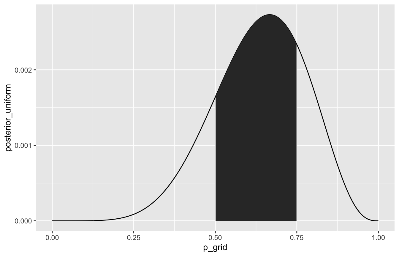


samples_tidy %>% 
  count(p_grid > 0.5 & p_grid < 0.75) %>% 
  mutate(probability = n / sum(n))
## # A tibble: 2 × 3
##   `p_grid > 0.5 & p_grid < 0.75`     n probability
##   <lgl>                          <int>       <dbl>
## 1 FALSE                           4000         0.4
## 2 TRUE                            6000         0.6

3.2.2: Intervals of defined mass

Base R
Tidyverse

Lower 80% posterior probability lies below this number:

quantile(samples, 0.8)
##      80% 
## 0.759576

Middle 80% posterior probability lies between these numbers:

quantile(samples, c(0.1, 0.9))
##       10%       90% 
## 0.4448445 0.8106911

50% percentile interval vs. 50% HPDI

quantile(samples, c(0.25, 0.75))
##       25%       75% 
## 0.5416292 0.7387989
rethinking::HPDI(samples, prob = 0.5)
##      |0.5      0.5| 
## 0.5659566 0.7592759

Lower 80% posterior probability lies below this number:

samples_tidy %>% 
  summarize(`80th percentile` = quantile(p_grid, 0.8))
## # A tibble: 1 × 1
##   `80th percentile`
##               <dbl>
## 1             0.762

Middle 80% posterior probability lies between these numbers:

samples_tidy %>% 
  summarize(q = c(0.1, 0.9), percentile = quantile(p_grid, q)) %>% 
  pivot_wider(names_from = q, values_from = percentile)
## # A tibble: 1 × 2
##   `0.1` `0.9`
##   <dbl> <dbl>
## 1  0.45 0.811

50% percentile interval vs. 50% HPDI

samples_tidy %>% 
  summarize(q = c(0.25, 0.75), 
            percentile = quantile(p_grid, q),
            hpdi = HDInterval::hdi(p_grid, 0.5))
## # A tibble: 2 × 3
##       q percentile  hpdi
##   <dbl>      <dbl> <dbl>
## 1  0.25      0.544 0.563
## 2  0.75      0.742 0.756

3.2.3: Point estimates

Base R
Tidyverse

mean(samples)
## [1] 0.6352952
median(samples)
## [1] 0.6448645

samples_tidy %>% 
  summarize(mean = mean(p_grid),
            median = median(p_grid))
## # A tibble: 1 × 2
##    mean median
##   <dbl>  <dbl>
## 1 0.638  0.646

3.3: Sampling to simulate prediction

Base R

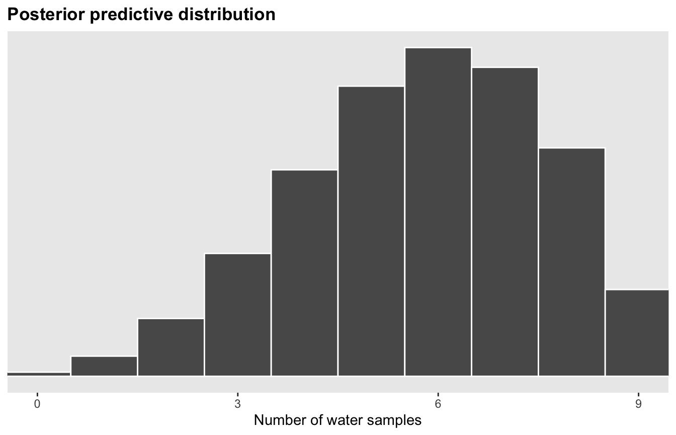
We can use the uncertainty inherent in the sampling distributions from above to generate a posterior predictive distribution, based on a 9-toss situation:

# Posterior predictive distribution
posterior_predictive_dist <- rbinom(10000, size = 9, prob = samples)
hist(posterior_predictive_dist, breaks = 0:9)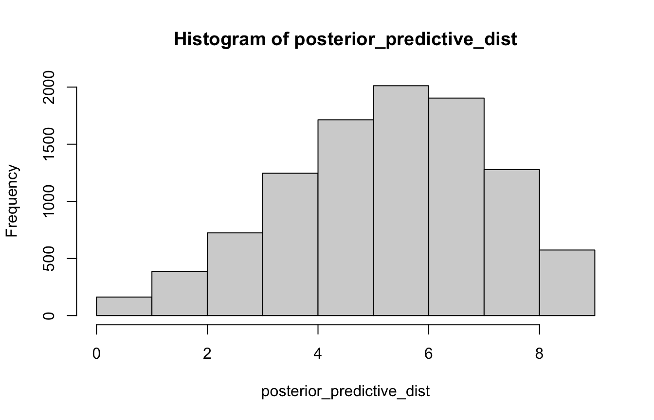

Tidyverse style

# Generate 100,000 samples from the posterior
samples_tidy <- globe_tossing %>% 
  slice_sample(n = 100000, weight_by = posterior_uniform, replace = T)
#
samples_tidy %>% 
  mutate(sample_number = 1:n()) %>% 
  ggplot(aes(x = sample_number, y = p_grid)) +
  geom_point(alpha = 0.05) +
  labs(title = "100,000 posterior samples", x = "Sample number")
#
samples_tidy %>% 
  ggplot(aes(x = p_grid)) +
  geom_density(fill = "grey50", color = NA) +
  labs(title = "Distribution of 100,000 posterior samples")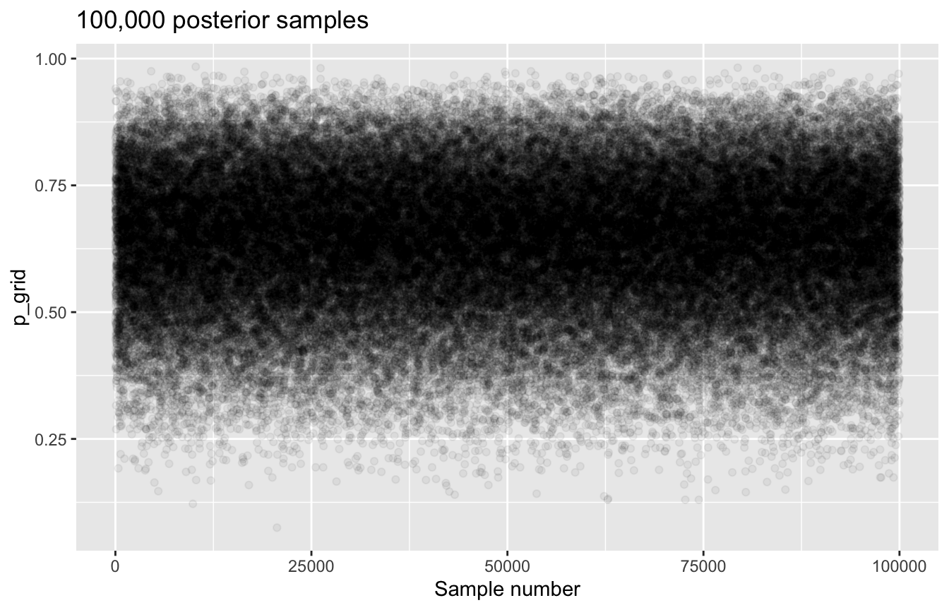

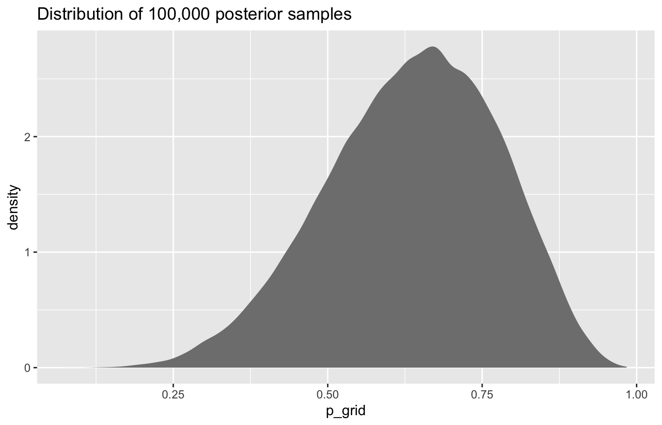
Figure 3.6 with ggplot

# Posterior probability
globe_smaller <- globe_tossing %>% 
  filter(p_grid %in% c(seq(0.1, 0.9, 0.1), 0.3))

panel_top <- globe_tossing %>% 
  ggplot(aes(x = p_grid, y = posterior_uniform)) + 
  geom_area(fill = "grey50", color = NA) +
  geom_segment(data = globe_smaller, aes(xend = p_grid, yend = 0, size = posterior_uniform)) +
  geom_point(data = globe_smaller) +
  scale_size_continuous(range = c(0, 1), guide = "none") +
  scale_x_continuous(breaks = seq(0, 1, 0.1)) +
  scale_y_continuous(NULL, breaks = NULL) +
  labs(x = "Proportion/probability of water",
       title = "Posterior probability") +
  theme(panel.grid = element_blank(),
        plot.title = element_text(face = "bold"))

# Sampling distributions
globe_sample_dists <- tibble(probability = seq(0.1, 0.9, 0.1)) %>% 
  mutate(draws = map(probability, ~{
    set.seed(1234)
    rbinom(10000, size = 9, prob = .x)
  })) %>% 
  unnest(draws) %>% 
  mutate(label = paste0("p = ", probability))

panel_middle <- ggplot(globe_sample_dists, aes(x = draws)) +
  geom_histogram(binwidth = 1, center = 0, color = "white", size = 0.1) +
  scale_x_continuous(breaks = seq(0, 9, 3)) +
  scale_y_continuous(breaks = NULL) +
  coord_cartesian(xlim = c(0, 9)) +
  labs(x = NULL, y = NULL, title = "Sampling distributions") +
  theme(panel.grid = element_blank(),
        plot.title = element_text(face = "bold")) +
  facet_wrap(vars(label), ncol = 9)

# Posterior predictive distribution
globe_samples <- globe_tossing %>% 
  slice_sample(n = 10000, weight_by = posterior_uniform, replace = TRUE) %>% 
  mutate(prediction = map_dbl(p_grid, rbinom, n = 1, size = 9))

panel_bottom <- globe_samples %>% 
  ggplot(aes(x = prediction)) +
  geom_histogram(binwidth = 1, center = 0, color = "white", size = 0.5) +
  scale_x_continuous(breaks = seq(0, 9, 3)) +
  scale_y_continuous(breaks = NULL) +
  coord_cartesian(xlim = c(0, 9)) +
  labs(x = "Number of water samples", y = NULL, title = "Posterior predictive distribution") +
  theme(panel.grid = element_blank(),
        plot.title = element_text(face = "bold"))

layout <- "
AAAAAAAAAAA
#BBBBBBBBB#
###CCCCC###
"

panel_top / panel_middle / panel_bottom +
  plot_layout(design = layout)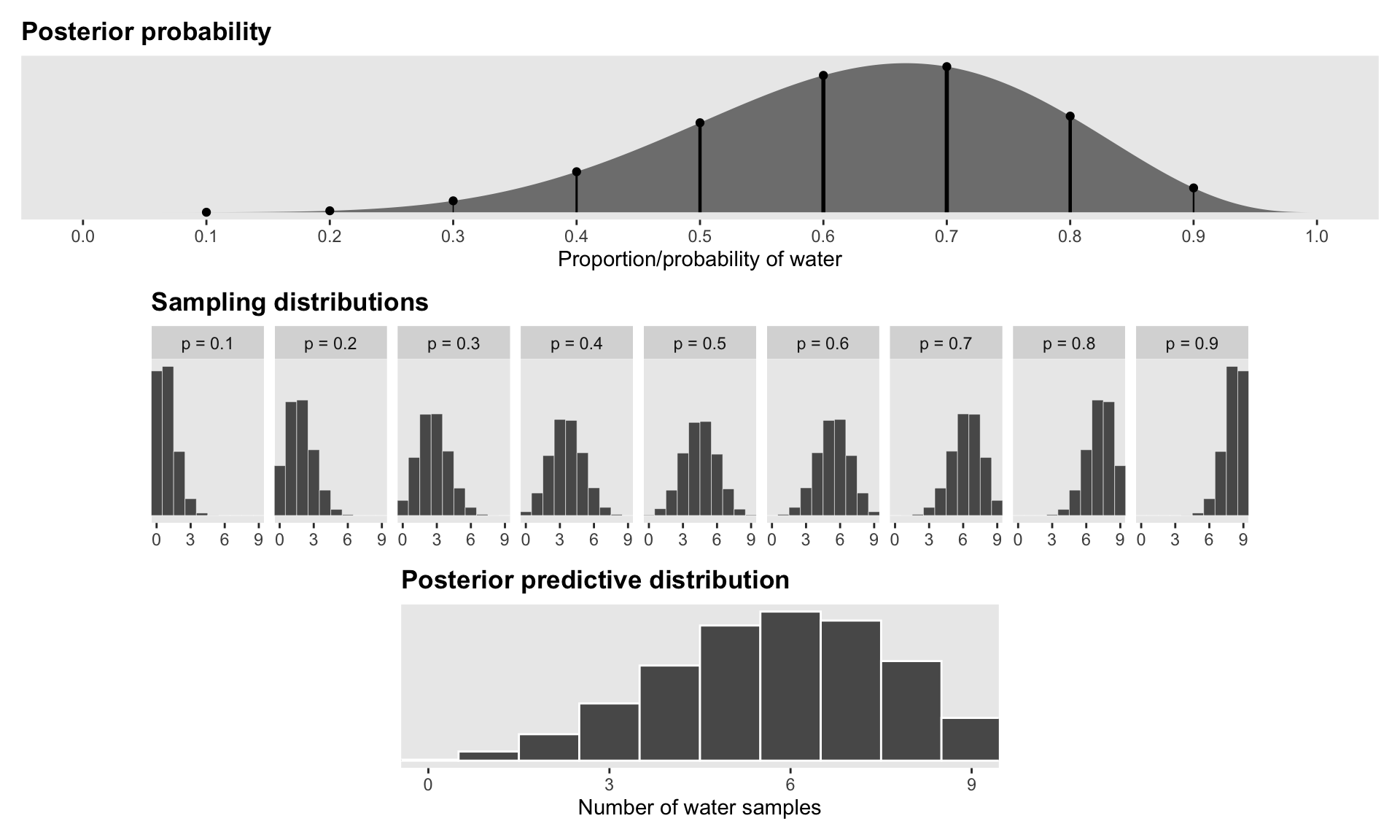

brms and tidybayes version of all this

Ooh neat, you can pass single values as data instead of a data frame! Everything else here looks like regular brms stuff.

model_globe <- brm(
  bf(water | trials(9) ~ 0 + Intercept),
  data = list(water = 6),
  family = binomial(link = "identity"),
  # Flat uniform prior
  prior(beta(1, 1), class = b, lb = 0, ub = 1),
  iter = 5000, warmup = 1000, seed = 1234,
  # TODO: Eventually switch to cmdstanr once this issue is fixed
  # https://github.com/quarto-dev/quarto-cli/issues/2258
  backend = "rstan", cores = 4
)
## Compiling Stan program...
## Trying to compile a simple C file
## Start sampling

Credible intervals / HPDI / etc.

# Using broom.mixed
tidy(model_globe, effects = "fixed",
     conf.level = 0.5, conf.method = "HPDinterval")
## # A tibble: 1 × 7
##   effect component term        estimate std.error conf.low conf.high
##   <chr>  <chr>     <chr>          <dbl>     <dbl>    <dbl>     <dbl>
## 1 fixed  cond      (Intercept)    0.639     0.137    0.568     0.761

# Using the posterior package
draws <- as_draws_array(model_globe)
summarize_draws(draws, default_summary_measures()) %>% 
  filter(variable == "b_Intercept")
## # A tibble: 1 × 7
##   variable     mean median    sd   mad    q5   q95
##   <chr>       <dbl>  <dbl> <dbl> <dbl> <dbl> <dbl>
## 1 b_Intercept 0.639  0.648 0.137 0.144 0.400 0.848

# Using tidybayes
# get_variables(model_globe)
model_globe %>% 
  spread_draws(b_Intercept) %>% 
  median_hdci(b_Intercept, .width = c(0.5, 0.89, 0.95))
## # A tibble: 3 × 6
##   b_Intercept .lower .upper .width .point .interval
##         <dbl>  <dbl>  <dbl>  <dbl> <chr>  <chr>    
## 1       0.648  0.568  0.761   0.5  median hdci     
## 2       0.648  0.430  0.864   0.89 median hdci     
## 3       0.648  0.374  0.892   0.95 median hdci

model_globe %>% 
  gather_draws(b_Intercept) %>% 
  ggplot(aes(x = .value, y = .variable)) +
  stat_halfeye()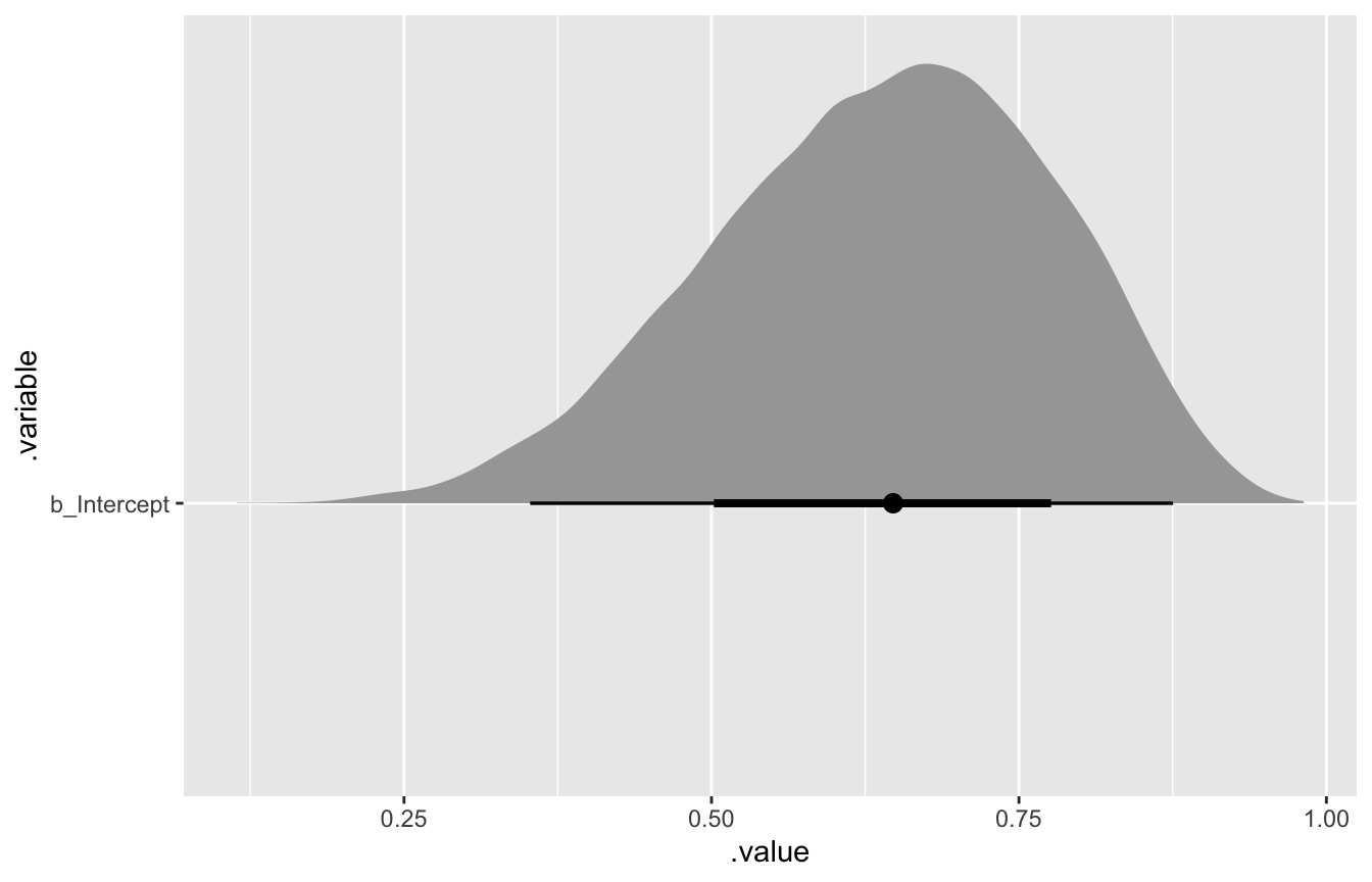

Predictions

model_globe %>% 
  predicted_draws(newdata = tibble(nothing = 1)) %>% 
  ggplot(aes(x = .prediction)) +
  geom_histogram(binwidth = 1, center = 0, color = "white", size = 0.5) +
  scale_x_continuous(breaks = seq(0, 9, 3)) +
  scale_y_continuous(breaks = NULL) +
  coord_cartesian(xlim = c(0, 9)) +
  labs(x = "Number of water samples", y = NULL, title = "Posterior predictive distribution") +
  theme(panel.grid = element_blank(),
        plot.title = element_text(face = "bold"))