library(tidyverse)
library(furrr)
library(ggdag)
library(ggraph)
library(patchwork)

# Parallel stuff
plan(multisession, workers = 4)

# Plot stuff
clrs <- MetBrewer::met.brewer("Lakota", 6)
theme_set(theme_bw())

# Seed stuff
set.seed(1234)Video #6 code
Good & bad controls
No code here; the lecture is a good overview of DAGs and good/bad controls.
Post-treatment mediator
If we have this DAG, where \(Z\) is a mediator between \(X\) and \(Y\), and \(u\) is some unobserved confounding, should we control for \(Z\)? No!
Code
dagify(
  Y ~ Z + u,
  Z ~ X + u,
  exposure = "X",
  outcome = "Y",
  latent = "u",
  coords = list(x = c(X = 1, Y = 4, Z = 2, u = 3),
                y = c(X = 1, Y = 1, Z = 1, u = 2))) %>%
  tidy_dagitty() %>%
  node_status() %>%
  as_tibble() %>%
  left_join(tribble(
    ~name, ~to, ~coef,
    "X",   "Z", 1,
    "u",   "Z", 1,
    "u",   "Y", 1,
    "Z",   "Y", 1
  ), by = c("name", "to")) %>%
  mutate(latent = status == "latent",
         latent = ifelse(is.na(latent), FALSE, latent)) %>%
  ggplot(aes(x = x, y = y, xend = xend, yend = yend)) +
  geom_dag_edges(aes(edge_linetype = latent, label = coef),
                 angle_calc = "along", label_dodge = grid::unit(10, 'points')) +
  geom_dag_point(aes(color = status)) +
  geom_dag_text(aes(label = name), size = 3.5, color = "white") +
  scale_color_manual(values = c(clrs[1], "grey50", clrs[4]),
                     na.value = "black", guide = "none") +
  scale_edge_linetype_manual(values = c("solid", "43"), guide = "none") +
  ylim(c(0.9, 2.1)) +
  theme_dag()
Here’s a simulation to show why. It uses completely random and independent values for \(X\) and \(u\), and \(Z\) and \(Y\) are determined by coefficients (1 in this case). When using the model Y ~ X, \(X\) has the correct coefficient (0); when using the model Y ~ X + Z, the coefficient for \(X\) is super wrong and negative:
n <- 100
bXZ <- 1
bZY <- 1

sim <- tibble(sim_id = 1:1000) %>%
  mutate(sim = future_map(sim_id, ~{
    tibble(
      X = rnorm(n),
      u = rnorm(n),
      Z = rnorm(n, bXZ*X + u),
      Y = rnorm(n, bZY*Z + u)
    )
  }, .options = furrr_options(seed = TRUE))) %>%
  mutate(bX = future_map_dbl(sim, ~coef(lm(Y ~ X, data = .))["X"]),
         bXZ = future_map_dbl(sim, ~coef(lm(Y ~ X + Z, data = .))["X"]))

sim %>%
  select(-sim) %>%
  pivot_longer(starts_with("b")) %>%
  mutate(correct = ifelse(name == "bX", "Correct", "Wrong"),
         name = recode(name, "bX" = "Y ~ X", "bXZ" = "Y ~ X + Z")) %>%
  ggplot(aes(x = value, color = name, linetype = correct)) +
  geom_density(size = 1) +
  scale_color_manual(values = c(clrs[5], clrs[2])) +
  scale_linetype_manual(values = c("solid", "dotted")) +
  xlim(c(-1.5, 2)) +
  labs(x = "β for X", linetype = NULL, color = NULL) +
  theme(legend.position = "bottom")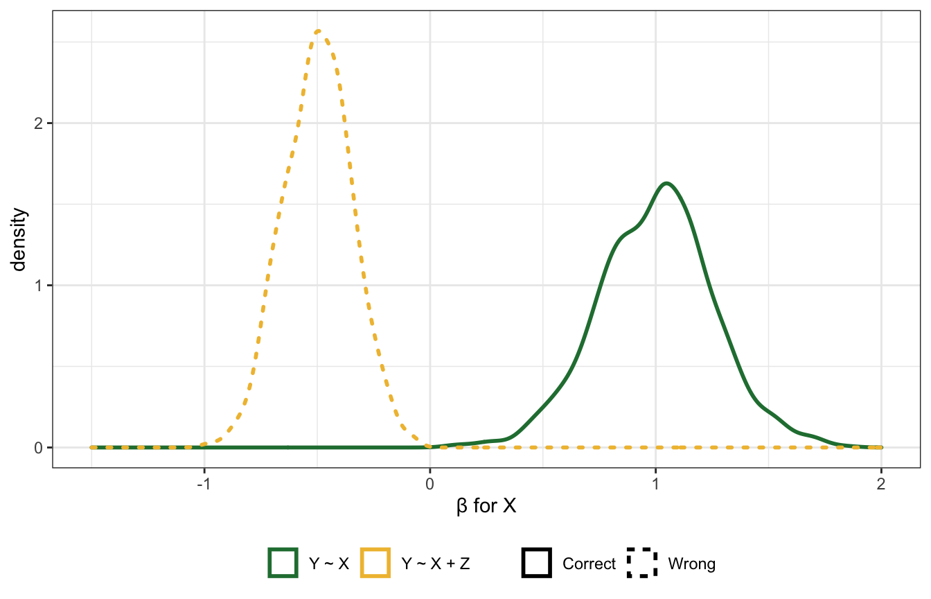
We can see the same thing even if the coefficient between \(Z\) and \(Y\) is set to zero:
Code
dagify(
  Y ~ Z + u,
  Z ~ X + u,
  exposure = "X",
  outcome = "Y",
  latent = "u",
  coords = list(x = c(X = 1, Y = 4, Z = 2, u = 3),
                y = c(X = 1, Y = 1, Z = 1, u = 2))) %>%
  tidy_dagitty() %>%
  node_status() %>%
  as_tibble() %>%
  left_join(tribble(
    ~name, ~to, ~coef,
    "X",   "Z", 1,
    "u",   "Z", 1,
    "u",   "Y", 1,
    "Z",   "Y", 0
  ), by = c("name", "to")) %>%
  mutate(latent = status == "latent",
         latent = ifelse(is.na(latent), FALSE, latent)) %>%
  ggplot(aes(x = x, y = y, xend = xend, yend = yend)) +
  geom_dag_edges(aes(edge_linetype = latent, label = coef),
                 angle_calc = "along", label_dodge = grid::unit(10, 'points')) +
  geom_dag_point(aes(color = status)) +
  geom_dag_text(aes(label = name), size = 3.5, color = "white") +
  scale_color_manual(values = c(clrs[1], "grey50", clrs[4]),
                     na.value = "black", guide = "none") +
  scale_edge_linetype_manual(values = c("solid", "43"), guide = "none") +
  ylim(c(0.9, 2.1)) +
  theme_dag()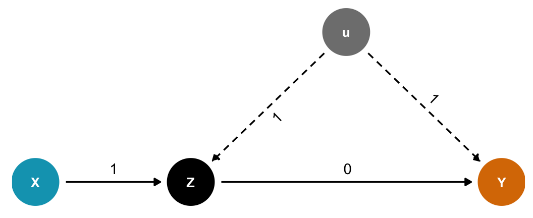
n <- 100
bXZ <- 1
bZY <- 0

sim <- tibble(sim_id = 1:1000) %>%
  mutate(sim = future_map(sim_id, ~{
    tibble(
      X = rnorm(n),
      u = rnorm(n),
      Z = rnorm(n, bXZ*X + u),
      Y = rnorm(n, bZY*Z + u)
    )
  }, .options = furrr_options(seed = TRUE))) %>%
  mutate(bX = future_map_dbl(sim, ~coef(lm(Y ~ X, data = .))["X"]),
         bXZ = future_map_dbl(sim, ~coef(lm(Y ~ X + Z, data = .))["X"]))

sim %>%
  select(-sim) %>%
  pivot_longer(starts_with("b")) %>%
  mutate(correct = ifelse(name == "bX", "Correct", "Wrong"),
         name = recode(name, "bX" = "Y ~ X", "bXZ" = "Y ~ X + Z")) %>%
  ggplot(aes(x = value, color = name, linetype = correct)) +
  geom_density(size = 1) +
  scale_color_manual(values = c(clrs[5], clrs[2])) +
  scale_linetype_manual(values = c("solid", "dotted")) +
  xlim(c(-1.5, 2)) +
  labs(x = "β for X", linetype = NULL, color = NULL) +
  theme(legend.position = "bottom")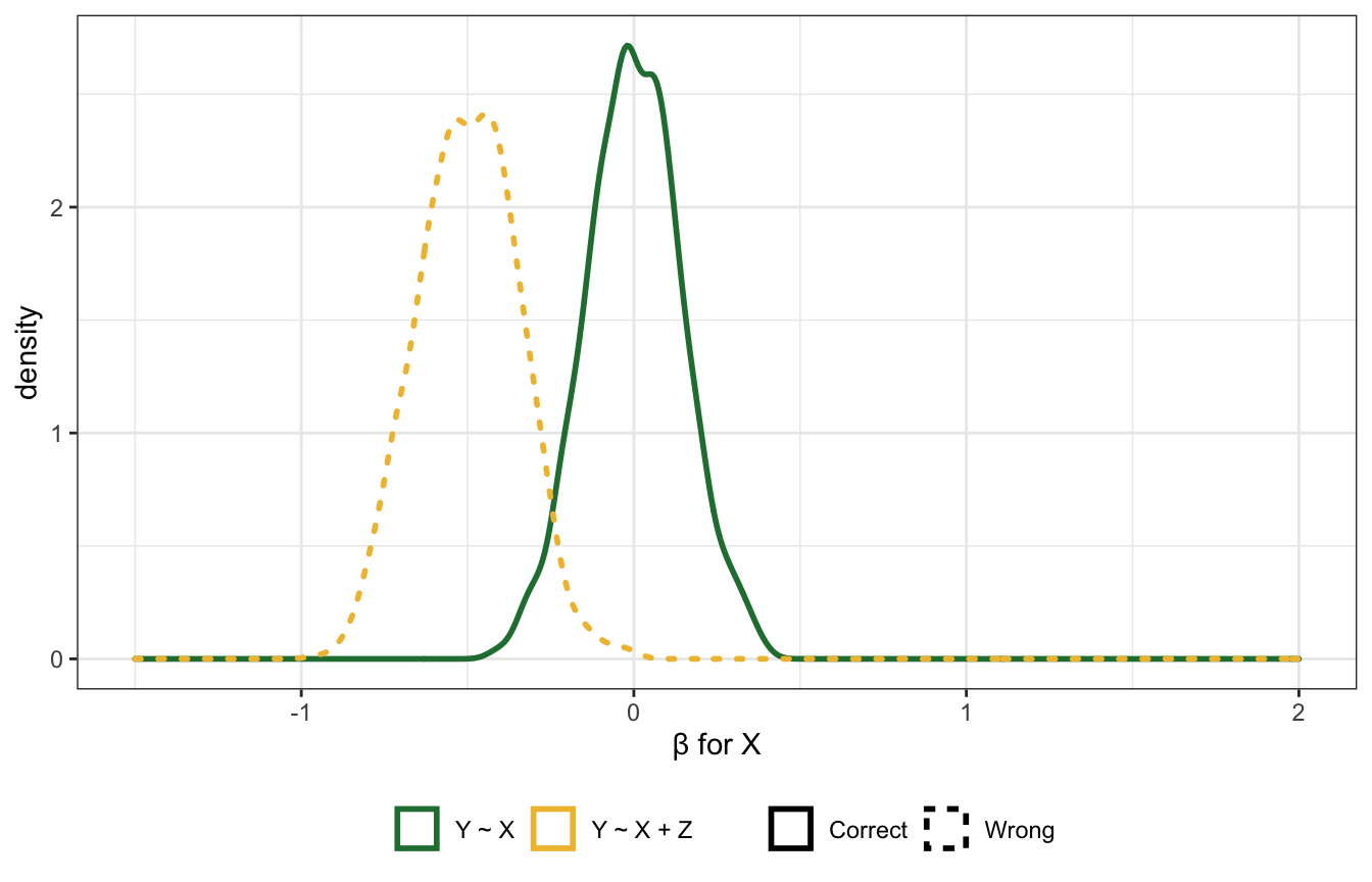
Case-control bias
Here \(Z\) comes after the outcome, like if \(X\) is education, \(Y\) is occupation, and \(Z\) is income. Should we control for \(Z\)? Surely that’s harmless?
Nope!
Code
dagify(
  Y ~ X,
  Z ~ Y,
  exposure = "X",
  outcome = "Y",
  coords = list(x = c(X = 1, Y = 2, Z = 3),
                y = c(X = 1, Y = 1, Z = 1))) %>%
  tidy_dagitty() %>%
  node_status() %>%
  as_tibble() %>%
  left_join(tribble(
    ~name, ~to, ~coef,
    "X",   "Y", 1,
    "Y",   "Z", 1
  ), by = c("name", "to")) %>%
  ggplot(aes(x = x, y = y, xend = xend, yend = yend)) +
  geom_dag_edges(aes(label = coef),
                 angle_calc = "along", label_dodge = grid::unit(10, 'points')) +
  geom_dag_point(aes(color = status)) +
  geom_dag_text(aes(label = name), size = 3.5, color = "white") +
  scale_color_manual(values = c(clrs[1], clrs[4]),
                     na.value = "black", guide = "none") +
  xlim(c(0.75, 3.25)) + ylim(c(0.9, 1.1)) +
  theme_dag()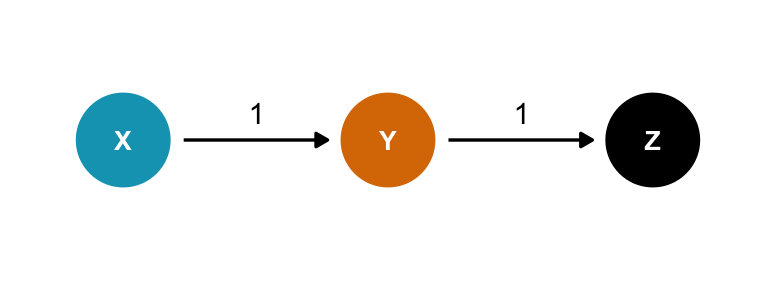
n <- 100
bXY <- 1
bYZ <- 1

sim <- tibble(sim_id = 1:1000) %>%
  mutate(sim = future_map(sim_id, ~{
    tibble(
      X = rnorm(n),
      Z = rnorm(n, bXY*X),
      Y = rnorm(n, bYZ*Z)
    )
  }, .options = furrr_options(seed = TRUE))) %>%
  mutate(bX = future_map_dbl(sim, ~coef(lm(Y ~ X, data = .))["X"]),
         bXZ = future_map_dbl(sim, ~coef(lm(Y ~ X + Z, data = .))["X"]))

sim %>%
  select(-sim) %>%
  pivot_longer(starts_with("b")) %>%
  mutate(correct = ifelse(name == "bX", "Correct", "Wrong"),
         name = recode(name, "bX" = "Y ~ X", "bXZ" = "Y ~ X + Z")) %>%
  ggplot(aes(x = value, color = name, linetype = correct)) +
  geom_density(size = 1) +
  scale_color_manual(values = c(clrs[5], clrs[2])) +
  scale_linetype_manual(values = c("solid", "dotted")) +
  xlim(c(-1, 2)) +
  labs(x = "β for X", linetype = NULL, color = NULL) +
  theme(legend.position = "bottom")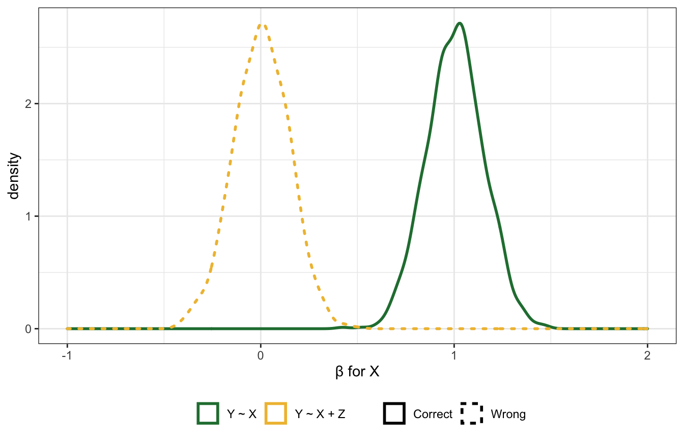
Precision parasite
Here \(Z\) comes before the treatment and doesn’t open any backdoors. Should we control for it? Again, it should be harmless?
In this case, it doesn’t distort the effect, but it does reduce the precision of the estimate
Code
dagify(
  Y ~ X,
  X ~ Z,
  exposure = "X",
  outcome = "Y",
  coords = list(x = c(X = 2, Y = 3, Z = 1),
                y = c(X = 1, Y = 1, Z = 1))) %>%
  tidy_dagitty() %>%
  node_status() %>%
  as_tibble() %>%
  left_join(tribble(
    ~name, ~to, ~coef,
    "X",   "Y", 1,
    "Z",   "X", 1
  ), by = c("name", "to")) %>%
  ggplot(aes(x = x, y = y, xend = xend, yend = yend)) +
  geom_dag_edges(aes(label = coef),
                 angle_calc = "along", label_dodge = grid::unit(10, 'points')) +
  geom_dag_point(aes(color = status)) +
  geom_dag_text(aes(label = name), size = 3.5, color = "white") +
  scale_color_manual(values = c(clrs[1], clrs[4]),
                     na.value = "black", guide = "none") +
  xlim(c(0.75, 3.25)) + ylim(c(0.9, 1.1)) +
  theme_dag()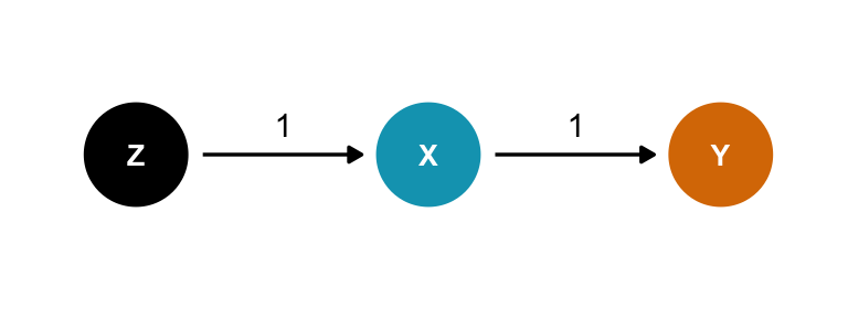
n <- 100
bZX <- 1
bXY <- 1

sim <- tibble(sim_id = 1:1000) %>%
  mutate(sim = future_map(sim_id, ~{
    tibble(
      Z = rnorm(n),
      X = rnorm(n, bZX*Z),
      Y = rnorm(n, bXY*X)
    )
  }, .options = furrr_options(seed = TRUE))) %>%
  mutate(bX = future_map_dbl(sim, ~coef(lm(Y ~ X, data = .))["X"]),
         bXZ = future_map_dbl(sim, ~coef(lm(Y ~ X + Z, data = .))["X"]))

sim %>%
  select(-sim) %>%
  pivot_longer(starts_with("b")) %>%
  mutate(correct = ifelse(name == "bX", "Correct", "Wrong"),
         name = recode(name, "bX" = "Y ~ X", "bXZ" = "Y ~ X + Z")) %>%
  ggplot(aes(x = value, color = name, linetype = correct)) +
  geom_density(size = 1) +
  scale_color_manual(values = c(clrs[5], clrs[2])) +
  scale_linetype_manual(values = c("solid", "dotted")) +
  xlim(c(0.5, 1.5)) +
  labs(x = "β for X", linetype = NULL, color = NULL) +
  theme(legend.position = "bottom")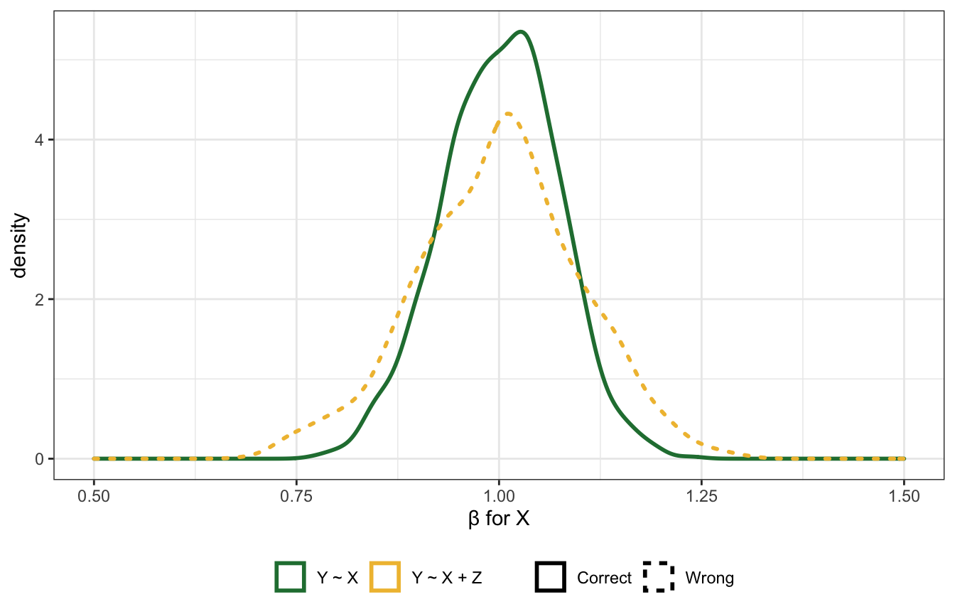
Bias amplification
Like the precision parasite situation, but with an unobserved confounder \(u\). Really bad stuff happens here (“something truly awful” in the lecture). The true coefficient between \(X\) and \(Y\) here is 0, but the estimate is wrong with both models!
Including causes of the exposure is generally a really bad idea. Covariation in \(X\) and \(Y\) requires variation in their causes, but within different levels of \(Z\) (since we’re stratifying by or adjusting for \(Z\)), there’s less variation in \(X\). That makes the unobserved \(u\) confounder more important when determining \(X\).
Code
dagify(
  Y ~ X + u,
  X ~ Z + u,
  exposure = "X",
  outcome = "Y",
  latent = "u",
  coords = list(x = c(X = 2, Y = 4, Z = 1, u = 3),
                y = c(X = 1, Y = 1, Z = 1, u = 2))) %>%
  tidy_dagitty() %>%
  node_status() %>%
  as_tibble() %>%
  left_join(tribble(
    ~name, ~to, ~coef,
    "X",   "Y", 0,
    "u",   "X", 1,
    "u",   "Y", 1,
    "Z",   "X", 1
  ), by = c("name", "to")) %>%
  mutate(latent = status == "latent",
         latent = ifelse(is.na(latent), FALSE, latent)) %>%
  ggplot(aes(x = x, y = y, xend = xend, yend = yend)) +
  geom_dag_edges(aes(edge_linetype = latent, label = coef),
                 angle_calc = "along", label_dodge = grid::unit(10, 'points')) +
  geom_dag_point(aes(color = status)) +
  geom_dag_text(aes(label = name), size = 3.5, color = "white") +
  scale_color_manual(values = c(clrs[1], "grey50", clrs[4]),
                     na.value = "black", guide = "none") +
  scale_edge_linetype_manual(values = c("solid", "43"), guide = "none") +
  ylim(c(0.9, 2.1)) +
  theme_dag()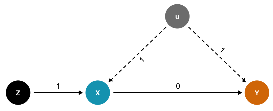
n <- 100
bZX <- 1
bXY <- 0

sim <- tibble(sim_id = 1:1000) %>%
  mutate(sim = future_map(sim_id, ~{
    tibble(
      Z = rnorm(n),
      u = rnorm(n),
      X = rnorm(n, bZX*Z + u),
      Y = rnorm(n, bXY*X + u)
    )
  }, .options = furrr_options(seed = TRUE))) %>%
  mutate(bX = future_map_dbl(sim, ~coef(lm(Y ~ X, data = .))["X"]),
         bXZ = future_map_dbl(sim, ~coef(lm(Y ~ X + Z, data = .))["X"]))

sim %>%
  select(-sim) %>%
  pivot_longer(starts_with("b")) %>%
  mutate(correct = ifelse(name == "bX", "Wrong", "Wrong but worse"),
         name = recode(name, "bX" = "Y ~ X", "bXZ" = "Y ~ X + Z")) %>%
  ggplot(aes(x = value, color = name, linetype = correct)) +
  geom_density(size = 1) +
  scale_color_manual(values = c(clrs[5], clrs[2])) +
  scale_linetype_manual(values = c("dashed", "dotted")) +
  geom_vline(xintercept = 0) +
  annotate(geom = "text", x = -0.02, y = 2.5, label = "Actual value", angle = 90) +
  xlim(c(-0.15, 1)) +
  labs(x = "β for X", linetype = NULL, color = NULL) +
  theme(legend.position = "bottom")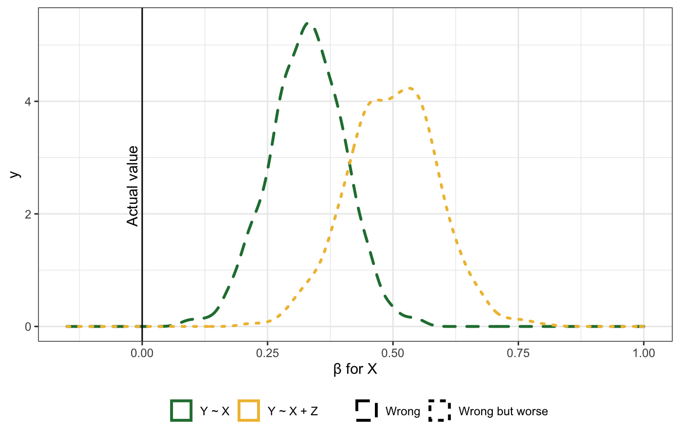
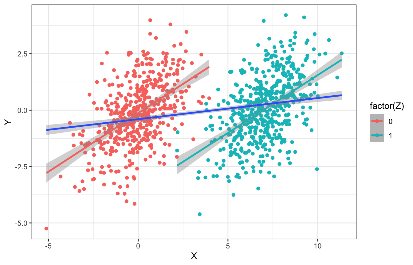
This whole idea that controlling for \(Z\) in the presence of unmeasured confounding amplifies the bias is really weird. Here’s another simulation from McElreath’s slides, where there is no relationship between \(X\) and \(Y\). There is a slight relationship between \(X\) and \(Y\) because of \(u\), but once we stratify by \(Z\), those slopes get bigger within each group!
tibble(Z = rbinom(1000, 1, 0.5),
       u = rnorm(1000)) %>%
  mutate(X = rnorm(1000, 7*Z + u),
         Y = rnorm(1000, 0*X + u)) %>%
  ggplot(aes(x = X, y = Y, color = factor(Z))) +
  geom_point() +
  geom_smooth(method = "lm") +
  geom_smooth(aes(color = NULL), method = "lm")